2.11: Variable Separation – Spherical Coordinates

The spherical coordinates are very important in physics, because of the (at least approximate) spherical symmetry of many physical objects – from nuclei and atoms, to water drops in clouds, to planets and stars. Let us again require each component \(\ \phi_{k}\) of Eq. (84) to satisfy the Laplace equation. Using the full expression for the Laplace operator in spherical coordinates,⁵¹ we get

\[\ \frac{1}{r^{2}} \frac{\partial}{\partial r}\left(r^{2} \frac{\partial \phi_{k}}{\partial r}\right)+\frac{1}{r^{2} \sin \theta} \frac{\partial}{\partial \theta}\left(\sin \theta \frac{\partial \phi_{k}}{\partial \theta}\right)+\frac{1}{r^{2} \sin ^{2} \theta} \frac{\partial^{2} \phi_{k}}{\partial \varphi^{2}}=0.\tag{2.161}\]

Let us look for a solution of this equation in the following variable-separated form:

\[\ \phi_{k}=\frac{\mathcal{R}(r)}{r} \mathcal{P}(\cos \theta) \mathcal{F}(\varphi),\tag{2.162}\]

Separating the variables one by one, starting from \(\ \varphi\), just like this has been done in cylindrical coordinates, we get the following equations for the partial functions participating in this solution:

\[\ \frac{d^{2} \mathcal{R}}{d r^{2}}-\frac{l(l+1)}{r^{2}} \mathcal{R}=0,\tag{2.163}\]

\[\ \frac{d}{d \xi}\left[\left(1-\xi^{2}\right) \frac{d \mathcal{P}}{d \xi}\right]+\left[l(l+1)-\frac{\nu^{2}}{1-\xi^{2}}\right] \mathcal{P}=0,\tag{2.164}\]

\[\ \frac{d^{2} \mathcal{F}}{d \varphi^{2}}+\nu^{2} \mathcal{F}=0,\tag{2.165}\]

where \(\ \xi \equiv \cos \theta\) is a new variable used in lieu of \(\ \theta\) (so that \(\ -1 \leq \xi \leq+1\)), while \(\ \nu^{2}\) and \(\ l(l+1)\) are the separation constants. (The reason for selection of the latter one in this form will be clear in a minute.)

One can see that Eq. (165) is very simple, and is absolutely similar to the Eq. (107) we have got for the cylindrical coordinates. Moreover, the equation for the radial functions is simpler than in the cylindrical coordinates. Indeed, let us look for its partial solution in the form \(\ c r^{\alpha}\) – just as we have done with Eq. (106). Plugging this solution into Eq. (163), we immediately get the following condition on the parameter \(\ \alpha\):

\[\ \alpha(\alpha-1)=l(l+1).\tag{2.166}\]

This quadratic equation has two roots, \(\ \alpha=l+1\) and \(\ \alpha=-l\), so that the general solution to Eq. (163) is

\[\ \mathcal{R}=a_{l} r^{l+1}+\frac{b_{l}}{r^{l}}.\tag{2.167}\]

However, the general solution of Eq. (164) (called either the general or associated Legendre equation) cannot be expressed via what is usually called elementary functions.⁵² Let us start its discussion from the axially-symmetric case when \(\ \partial \phi / \partial \varphi=0\). This means \(\ \mathcal{F}(\varphi)=\text { const }\), and thus \(\ \nu=0\), so that Eq. (164) is reduced to the so-called Legendre differential equation:

Legendre equation

\[\ \frac{d}{d \xi}\left[\left(1-\xi^{2}\right) \frac{d \mathcal{P}}{d \xi}\right]+l(l+1) \mathcal{P}=0.\tag{2.168}\]

One can readily check that the solutions of this equation for integer values of \(\ l\) are specific (Legendre) polynomials⁵³ that may be described by the following Rodrigues’ formula:

Legendre polynomials

\[\ \mathcal{P}_{l}(\xi)=\frac{1}{2^{l} l !} \frac{d^{l}}{d \xi^{l}}\left(\xi^{2}-1\right)^{l}, \quad l=0,1,2, \ldots.\tag{2.169}\]

As this formula shows, the first few Legendre polynomials are pretty simple:

\[\ \begin{aligned}
&\mathcal{P}_{0}(\xi)=1, \\
&\mathcal{P}_{1}(\xi)=\xi, \\
&\mathcal{P}_{2}(\xi)=\frac{1}{2}\left(3 \xi^{2}-1\right), \\
&\mathcal{P}_{3}(\xi)=\frac{1}{2}\left(5 \xi^{3}-3 \xi\right), \\
&\mathcal{P}_{4}(\xi)=\frac{1}{8}\left(35 \xi^{4}-30 \xi^{2}+3\right), . .,
\end{aligned}\tag{2.170}\]

though such explicit expressions become more and more bulky as \(\ l\) is increased. As Fig. 23 shows, all these polynomials, which are defined on the [-1, +1] segment, end at the same point: \(\ \mathcal{P}_{l}(+1)=+1\), while starting either at the same point or at the opposite point: \(\ P_{l}(-1)=(-1)^{l}\). Between these two end points, the \(\ l^{\text {th }}\) polynomial has \(\ l\) zeros. It is straightforward to use Eq. (169) for proving that these polynomials form a full, orthogonal set of functions, with the following normalization rule:

\[\ \int_{-1}^{+1} \mathcal{P}_{l}(\xi) \mathcal{P}_{l^{\prime}}(\xi) d \xi=\frac{2}{2 l+1} \delta_{l l^{\prime}},\tag{2.171}\]

so that any function \(\ f(\xi)\) defined on the segment [-1, +1] may be represented as a unique series over the polynomials.⁵⁴

Thus, taking into account the additional division by \(\ r\) in Eq. (162), the general solution of any axially-symmetric Laplace problem may be represented as

Variable separation in spherical coordinates (for axial symmetry)

\[\ \phi(r, \theta)=\sum_{l=0}^{\infty}\left(a_{l} r^{l}+\frac{b_{l}}{r^{l+1}}\right) \mathcal{P}_{l}(\cos \theta).\tag{2.172}\]

Note a strong similarity between this solution and Eq. (112) for the 2D Laplace problem in the polar coordinates. However, besides the difference in the angular functions, there is also a difference (by one) in the power of the second radial function, and this difference immediately shows up in problem solutions.

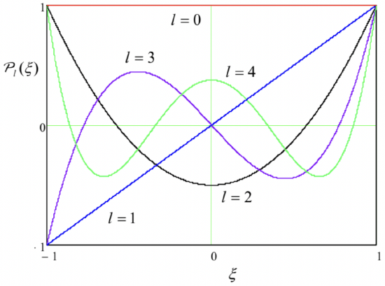Fig. 2.23. A few lowest Legendre polynomials \(\ P_{l}(\xi)\).

Indeed, let us solve a problem similar to that shown in Fig. 15: find the electric field around a conducting sphere of radius \(\ R\), placed into an initially uniform external field \(\ \mathbf{E}_{0}\) (whose direction I will now take for the z-axis) – see Fig. 24a.

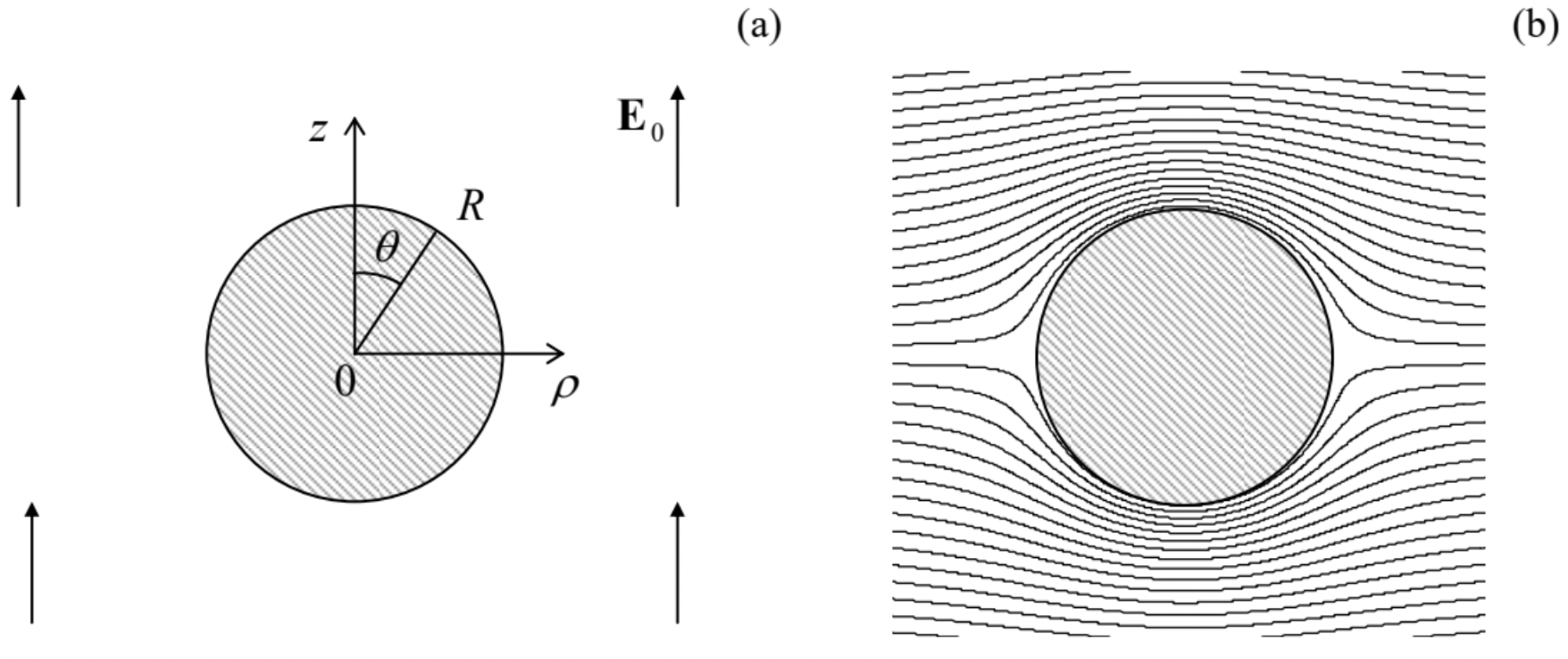Fig. 2.24. Conducting sphere in a uniform electric field: (a) the problem’s geometry, and (b) the equipotential surface pattern given by Eq. (176). The pattern is qualitatively similar but quantitatively different from that for the conducting cylinder in a perpendicular field – cf. Fig. 15.

If we select the arbitrary constant in the electrostatic potential so that \(\ \left.\phi\right|_{z=0}=0\), then in Eq. (172) we should take \(\ a_{0}=b_{0}=0\). Now, just as has been argued for the cylindrical case, at \(\ r>>R\) the potential should approach that of the uniform field:

\[\ \phi \rightarrow-E_{0} z=-E_{0} r \cos \theta,\tag{2.173}\]

so that in Eq. (172), only one of the coefficients \(\ a_{l}\) survives: \(\ a_{l}=-E_{0} \delta_{l, 1}\). As a result, from the boundary condition on the surface, \(\ \phi(R, \theta)=0\), we get the following equation for the coefficients \(\ b_{l}\):

\[\ \left(-E_{0} R+\frac{b_{1}}{R^{2}}\right) \cos \theta+\sum_{l \geq 2} \frac{b_{l}}{R^{l+1}} \mathcal{P}_{l}(\cos \theta)=0.\tag{2.174}\]

Now repeating the argumentation that led to Eq. (117), we may conclude that Eq. (174) is satisfied if

\[\ b_{l}=E_{0} R^{3} \delta_{l, 1},\tag{2.175}\]

so that, finally, Eq. (172) is reduced to

\[\ \phi=-E_{0}\left(r-\frac{R^{3}}{r^{2}}\right) \cos \theta.\tag{2.176}\]

This distribution, shown in Fig. 24b, is very much similar to Eq. (117) for the cylindrical case (cf. Fig. 15b, with the account for a different plot orientation), but with a different power of the radius in the second term. This difference leads to a quantitatively different distribution of the surface electric field:

\[\ E_{n}=-\left.\frac{\partial \phi}{\partial r}\right|_{r=R}=3 E_{0} \cos \theta,\tag{2.177}\]

so that its maximal value is a factor of 3 (rather than 2) larger than the external field.

Now let me briefly (mostly just for the reader’s reference) mention the Laplace equation solutions in the general case – with no axial symmetry). If the free space surrounds the origin from all sides, the solutions to Eq. (165) have to be \(\ 2 \pi\)-periodic, and hence \(\ \nu=n=0, \pm 1, \pm 2, \ldots\) Mathematics says that Eq. (164) with integer \(\ \nu=n\) and a fixed integer \(\ l\) has a solution only for a limited range of \(\ n\):⁵⁵

\[\ -l \leq n \leq+l.\tag{2.178}\]

These solutions are called the associated Legendre functions (generally, they are not polynomials!) For \(\ n \geq 0\), these functions may be defined via the Legendre polynomials, using the following formula:⁵⁶

\[\ \mathcal{P}_{l}^{n}(\xi)=(-1)^{n}\left(1-\xi^{2}\right)^{n / 2} \frac{d^{n}}{d \xi^{n}} \mathcal{P}_{l}(\xi).\tag{2.179}\]

On the segment \(\ \xi \in[-1,+1]\), each set of the associated Legendre functions with a fixed index \(\ n\) and non-negative values of \(\ l\) form a full, orthogonal set, with the normalization relation,

\[\ \int_{-1}^{+1} \mathcal{P}_{l}^{n}(\xi) \mathcal{P}_{l^{\prime}}^{n}(\xi) d \xi=\frac{2}{2 l+1} \frac{(l+n) !}{(l-n) !} \delta_{l l^{\prime}},\tag{2.180}\]

that is evidently a generalization of Eq. (171).

Since these relations may seem a bit intimidating, let me write down explicit expressions for a few \(\ \mathcal{P}_{l}^{n}(\cos \theta)\) with the lowest values of \(\ l\) and n \(\ \geq 0\), which are most important for applications.

\[\ l=0: \quad \mathcal{P}_{0}^{0}(\cos \theta)=1 ;\tag{2.181}\]

\[\ l=1: \quad\left\{\begin{array}{l}
\mathcal{P}_{1}^{0}(\cos \theta)=\cos \theta, \\
\mathcal{P}_{1}^{1}(\cos \theta)=-\sin \theta;
\end{array}\right.\tag{2.182}\]

\[\ l=2:\left\{\begin{array}{l}
\mathcal{P}_{2}^{0}(\cos \theta)=\left(3 \cos ^{2} \theta-1\right) / 2, \\
\mathcal{P}_{2}^{1}(\cos \theta)=-2 \sin \theta \cos \theta, \\
\mathcal{P}_{2}^{2}(\cos \theta)=-3 \cos ^{2} \theta.
\end{array}\right.\tag{2.183}\]

The reader should agree there is not much to fear in these functions – they are just certain sums of products of functions \(\ \cos \theta \equiv \xi\) and \(\ \sin \theta \equiv\left(1-\xi^{2}\right)^{1 / 2}\). Fig. 25 below shows the plots of a few lowest functions \(\ \mathcal{P}_{l}^{n}(\xi)\).

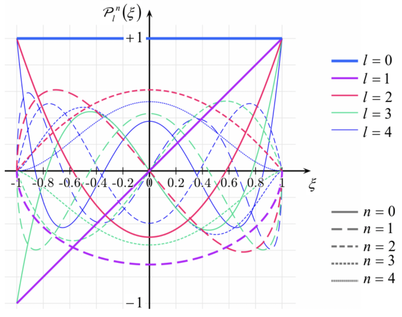Fig. 2.25. A few lowest associated Legendre functions. (Adapted from an original by Geek3, available at https://en.Wikipedia.org/wiki/Associ...re_polynomials, under the GNU Free Documentation License.)

Using the associated Legendre functions, the general solution (162) to the Laplace equation in the spherical coordinates may be expressed as

Variable separation in spherical coordinates (general case)

\[\ \phi(r, \theta, \varphi)=\sum_{l=0}^{\infty}\left(a_{l} r^{l}+\frac{b_{l}}{r^{l+1}}\right) \sum_{n=0}^{l} \mathcal{P}_{l}^{n}(\cos \theta) \mathcal{F}_{n}(\varphi), \quad \mathcal{F}_{n}(\varphi)=c_{n} \cos n \varphi+s_{n} \sin n \varphi.\tag{2.184}\]

Since the difference between the angles \(\ \theta\) and \(\ \varphi\) is somewhat artificial, physicists prefer to think not about the functions \(\ \mathcal{P}\) and \(\ \mathcal{F}\) in separation, but directly about their products that participate in this solution.⁵⁷

As a rare exception for my courses, to save time, I will skip giving an example of using the associated Legendre functions in electrostatics, because quite a few examples of these functions’ applications will be given in the quantum mechanics part of this series.

---

Reference

⁵¹ See, e.g., MA Eq. (10.9).

⁵² Actually, there is no generally accepted line between the “elementary” and “special” functions.

⁵³ Just for the reference: if l is not an integer, the general solution of Eq. (2.168) may be represented as a linear combination of the so-called Legendre functions (not polynomials!) of the first and second kind, \(\ \mathcal{P}_{1}(\xi)\) and \(\ Q_{l}(\xi)\).

⁵⁴ This is why, at least for the purposes of this course, there is no good reason for pursuing (more complex) solutions to Eq. (168) for non-integer values of \(\ l\), mentioned in the previous footnote.

⁵⁵ In quantum mechanics, the letter n is typically reserved used for the “principal quantum number”, while the azimuthal functions are numbered by index \(\ m\). However, here I will keep using \(\ n\) as their index because for this course’s purposes, this seems more logical in the view of the similarity of the spherical and cylindrical functions.

⁵⁶ Note that some texts use different choices for the front factor (called the Condon-Shortley phase) in the functions \(\ \mathcal{P}_{l}^{m}\), which do not affect the final results for the spherical harmonics \(\ Y_{l}^{m}\).

⁵⁷ In quantum mechanics, it is more convenient to use a slightly different, alternative set of basic functions of the same problem, namely the following complex functions called the spherical harmonics:

\(\ Y_{l}^{n}(\theta, \varphi) \equiv\left[\frac{2 l+1}{4 \pi} \frac{(l-n) !}{(l+n) !}\right]^{1 / 2} \mathcal{P}_{l}^{n}(\cos \theta) e^{i n \varphi},\)

which are defined for both positive and negative \(\ n\) (within the limits \(\ -l \leq n \leq+l\)) – see, e.g., QM Secs. 3.6 and 5.6. (Note again that in that field, the index \(\ n\) is traditionally denoted as \(\ m\), and called the magnetic quantum number.)