8.2: Electric Dipole Radiation

Consider again the problem that was discussed in electrostatics (Sec. 3.1), namely the field of a localized source with linear dimensions \(\ a<<r\) (see Fig. 1 again), but now with time-dependent charge and/or current distributions. Using the arguments of that discussion, in particular the condition expressed by Eq. (3.1), \(\ r^{\prime}<<r\), we may apply the Taylor expansion (3.3), truncated to two leading terms,

\[\ f(\mathbf{R})=f(\mathbf{r})-\mathbf{r}^{\prime} \cdot \nabla f(\mathbf{r})+\ldots,\tag{8.18}\]

to the scalar function \(\ f(\mathbf{R}) \equiv R\) (for which \(\ \nabla f(\mathbf{r})=\nabla R=\mathbf{n}\), where \(\ \mathbf{n} \equiv \mathbf{r} / r\) is the unit vector directed toward the observation point – see Fig. 1) to approximate the distance \(\ R\) as

\[\ R \approx r-\mathbf{r}^{\prime} \cdot \mathbf{n}.\tag{8.19}\]

In each of the retarded potential formulas (17), \(\ R\) participates in two places: in the denominator and in the source’s time argument. If \(\ \rho\) and \(\ \mathbf{j}\) change in time on the scale \(\ \sim 1 / \omega\), where \(\ \omega\) is some characteristic frequency, then any change of the argument \(\ (t-R / \nu)\) on that time scale, for example due to a change of \(\ R\) on the spatial scale \(\ \sim \nu / \omega=1 / k\), may substantially change these functions. Thus, the expansion (19) may be applied to \(\ R\) in the argument \(\ (t-R / \nu)\) only if \(\ k a<<1\), i.e. if the system’s size \(\ a\) is much smaller than the radiation wavelength \(\ \lambda=2 \pi / k\). On the other hand, the function \(\ 1/R\) changes relatively slowly, and for it even the first term of the expansion (19) gives a good approximation as soon as \(\ a<<r\), \(\ R\). In this approximation, Eq. (17a) yields

\[\ \phi(\mathbf{r}, t) \approx \frac{1}{4 \pi \varepsilon r} \int \rho\left(\mathbf{r}^{\prime}, t-\frac{R}{\nu}\right) d^{3} r^{\prime} \equiv \frac{1}{4 \pi \varepsilon r} Q\left(t-\frac{R}{\nu}\right),\tag{8.20}\]

where \(\ Q(t)\) is the net electric charge of the localized system. Due to the charge conservation, this charge cannot change with time, so that the approximation (20) describes just a static Coulomb field of our localized source, rather than a radiated wave.

Let us, however, apply a similar approximation to the vector potential (17b):

\[\ \mathbf{A}(\mathbf{r}, t) \approx \frac{\mu}{4 \pi r} \int \mathbf{j}\left(\mathbf{r}^{\prime}, t-\frac{R}{\nu}\right) d^{3} r^{\prime}.\tag{8.21}\]

According to Eq. (5.87), the right-hand side of this expression vanishes in statics, but in dynamics, this is no longer true. For example, if the current is due to a non-relativistic motion⁶ of a system of point charges \(\ q_{k}\), we can write

\[\ \int \mathbf{j}\left(\mathbf{r}^{\prime}, t\right) d^{3} r^{\prime}=\sum_{k} q_{k} \dot{\mathbf{r}}_{k}(t)=\frac{d}{d t} \sum_{k} q_{k} \mathbf{r}_{k}(t) \equiv \dot{\mathbf{p}}(t),\tag{8.22}\]

where \(\ \mathbf{p}(t)\) is the dipole moment of the localized system, defined by Eq. (3.6). Now, after the integration, we may keep only the first term of the approximation (19) in the argument \(\ (t-R / \nu)\) as well, getting

\[\ \mathbf{A}(\mathbf{r}, t) \approx \frac{\mu}{4 \pi r} \dot{\mathbf{p}}\left(t-\frac{r}{\nu}\right), \quad \text { for } a<<R, \frac{1}{k}.\tag{8.23}\]

Let us analyze what exactly this result describes. The second of Eqs. (1) allows us to calculate the magnetic field by the spatial differentiation of A. At large distances \(\ r >> \lambda\) (i.e. in the so-called far-field zone), where Eq. (23) describes a virtually plane wave, the main contribution into this derivative is given by the dipole moment factor:

\[\ \text{Far-field wave}\quad\quad\quad\quad \mathbf{B}(\mathbf{r}, t)=\frac{\mu}{4 \pi r} \nabla \times \dot{\mathbf{p}}\left(t-\frac{r}{\nu}\right)=-\frac{\mu}{4 \pi r \nu} \mathbf{n} \times \ddot{\mathbf{p}}\left(t-\frac{r}{\nu}\right).\tag{8.24}\]

This expression means that the magnetic field, at the observation point, is perpendicular to the vectors n and (the retarded value of) \(\ \ddot{\mathbf{p}}\), and its magnitude is

\[\ B=\frac{\mu}{4 \pi r \nu} \ddot{p}\left(t-\frac{r}{\nu}\right) \sin \Theta, \quad \text { i.e. } H=\frac{1}{4 \pi r \nu} \ddot{p}\left(t-\frac{r}{\nu}\right) \sin \Theta,\tag{8.25}\]

where \(\ \Theta\) is the angle between those two vectors – see Fig. 2.⁷

Fig. 8.2. Far-fields of a localized source, contributing to its electric dipole radiation.

The most important feature of this result is that the time-dependent field decreases very slowly (only as \(\ 1 / r\)) with the distance from the source, so that the radial component of the corresponding Poynting vector (7.9b),⁸

\[\ S_{r}=Z H^{2}=\frac{Z}{(4 \pi \nu r)^{2}}\left[\ddot{p}\left(t-\frac{r}{\nu}\right)\right]^{2} \sin ^{2} \Theta,\quad\quad\quad\quad \text{Instant power density}\tag{8.26}\]

drops as \(\ 1 / r^{2}\), i.e. the full instant power \(\ \mathscr{P}\) of the emitted wave,

\[\ \mathscr{P} \equiv \oint_{4 \pi} S_{r} r^{2} d \Omega=\frac{Z}{(4 \pi \nu)^{2}} \ddot{p}^{2} 2 \pi \int_{0}^{\pi} \sin ^{3} \Theta d \Theta=\frac{Z}{6 \pi \nu^{2}} \ddot{p}^{2}.\quad\quad\quad\quad\text{Larmor formula}\tag{8.27}\]

does not depend on the distance from the source – as it should for radiation.⁹

This is the famous Larmor formula¹⁰ for the electric dipole radiation; it is the dominating component of radiation by a localized system of charges – unless \(\ \ddot{\mathbf{p}}=0\). Please notice its angular dependence: the radiation vanishes at the axis of the retarded vector \(\ \ddot{\mathbf{p}}\) (where \(\ \Theta=0\)), and reaches its maximum in the plane perpendicular to that axis.

In order to find the average power, Eq. (27) has to be averaged over a sufficiently long time. In particular, if the source is monochromatic, \(\ \mathbf{p}(t)=\operatorname{Re}\left[\mathbf{p}_{\omega} \exp \{-i \omega t\}\right]\), with a time-independent vector \(\ \mathbf{p}_{\omega}\), such averaging may be carried out just over one period, giving an extra factor 2 in the denominator:

\[\ \overline{\mathscr{P}}=\frac{Z \omega^{4}}{12 \pi \nu^{2}}\left|p_{\omega}\right|^{2}.\quad\quad\quad\quad \text{Average radiation power}\tag{8.28}\]

The easiest application of this formula is to a point charge oscillating, with frequency \(\ \omega\), along a straight line (which we may take for the z-axis), with amplitude \(\ a\). In this case, \(\ \mathbf{p}=q z(t) \mathbf{n}_{z}=q a \operatorname{Re}[\exp \{-i\omega t\}]\mathbf{n}_z\), and if the charge velocity amplitude, \(\ a \omega\), is much less than the wave speed \(\ \nu\), we may use Eq. (28) with \(\ p_{\omega}=q a\), giving

\[\ \overline{\mathscr{P}}=\frac{Z q^{2} a^{2} \omega^{4}}{12 \pi \nu^{2}}.\tag{8.29}\]

Applied to an electron \(\ \left(q=-e \approx-1.6 \times 10^{-19} \mathrm{C}\right)\), initially rotating about a nucleus at an atomic distance \(\ a\sim 10^{-10} \mathrm{~m}\), the Larmor formula shows¹¹ that the energy loss due to the dipole radiation is so large that it would cause the electron to collapse on the atom’s nucleus in just \(\ \sim 10^{-10} \mathrm{~s}\). In the beginning of the 1900s, this classical result was one of the main arguments for the development of quantum mechanics, which prevents such collapse of electrons in their lowest-energy (ground) quantum state.

Another useful application of Eq. (28) is the radio wave radiation by a short, straight, symmetric antenna which is fed, for example, by a TEM transmission line such as a coaxial cable – see Fig. 3.

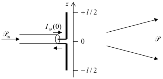Fig. 8.3. The dipole antenna.

The exact solution of this problem is rather complicated, because the law \(\ I_{\omega}(z)\) of the current variation along the antenna’s length should be calculated self consistently with the distribution of the electromagnetic field induced by the current in the surrounding space. (This fact is unfortunately ignored in some textbooks.) However, one may argue that at \(\ l<<\lambda\), the current should be largest in the feeding point (in Fig. 3, taken for \(\ z = 0\)), vanish at antenna’s ends \(\ (z=\pm l / 2)\), so that the linear function,

\[\ I_{\omega}(z)=I_{\omega}(0)\left(1-\frac{2}{l}|z|\right),\tag{8.30}\]

should give a good approximation of the actual distribution – as it indeed does. Now we can use the continuity equation \(\ \partial Q / \partial t=I\), i.e. \(\ -i \omega Q_{\omega}=I_{\omega}\), to calculate the complex amplitude \(\ Q \omega(z)=i I_{\omega}(z) \operatorname{sgn}(z) / \omega\) of the electric charge \(\ Q(z, t)=\operatorname{Re}\left[Q_{\omega} \exp \{-i \omega t\}\right]\) of the wire’s part beyond point \(\ z\), and from it, the amplitude of the linear density of charge

\[\ \lambda_{\omega}(z) \equiv \frac{d Q_{\omega}(z)}{d|z|}=-i \frac{2 I_{\omega}(0)}{\omega l} \operatorname{sgn} z.\tag{8.31}\]

From here, the dipole moment’s amplitude is

\[\ p_{\omega}=2 \int_{0}^{l / 2} \lambda_{\omega}(z) z d z=-i \frac{I_{\omega}(0)}{2 \omega} l,\tag{8.32}\]

so that Eq. (28) yields

\[\ \overline{\mathscr{P}}=Z \frac{\omega^{4}}{12 \pi \nu^{2}} \frac{\left|I_{\omega}(0)\right|^{2}}{4 \omega^{2}} l^{2}=\frac{Z(k l)^{2}}{24 \pi} \frac{\left|I_{\omega}(0)\right|^{2}}{2},\tag{8.33}\]

where \(\ k=\omega / \nu\). The analogy between this result and the dissipation power, \(\ \mathscr{P}=\operatorname{Re} Z\left|I_{\omega}\right|^{2} / 2\), in a lumped
linear circuit element, allows the interpretation of the first fraction in the last form of Eq. (33) as the real part of the antenna’s impedance:

\[\ \operatorname{Re} Z_{A}=Z \frac{(k l)^{2}}{24 \pi},\tag{8.34}\]

as felt by the transmission line.

According to Eq. (7.118), the wave traveling along the line toward the antenna is fully radiated, i.e. not reflected back, only if \(\ Z_{A}\) equals to of the line. As we know from Sec. 7.5 (and the solution of the related problems), for typical TEM lines, \(\ Z_{W} \sim Z_{0}\), while Eq. (34), which is only valid in the limit \(\ kl << 1\), shows that for radiation into free space \(\ \left(Z=Z_{0}\right)\), \(\ \operatorname{Re} Z_{A}\) is much less than \(\ \mathrm{Z}_{0}\). Hence to reach the impedance matching condition \(\ Z_{W}=Z_{A}\), the antenna’s length should be increased – as a more involved theory shows, to \(\ l \approx \lambda / 2\). However, in many cases, practical considerations make short antennas necessary. The example most often met nowadays is the cell phone antennas, which use frequencies close to 1 or 2 GHz, with free-space wavelengths \(\ \lambda\) between 15 and 30 cm, i.e. much larger than the phone size.¹² The quadratic dependence of the antenna’s efficiency on \(\ l\), following from Eq. (34), explains why every millimeter counts in the design of such antennas, and why their designs are carefully optimized using software packages for the (virtually exact) numerical solution of the Maxwell equations for the specific shape of the antenna and other phone parts.¹³

To conclude this section, let me note that if the wave source is not monochromatic, so that \(\ \mathbf{p}(t)\) should be represented as a Fourier series,

\[\ \mathbf{p}(t)=\operatorname{Re} \sum_{\omega} \mathbf{p}_{\omega} e^{-i \omega t},\tag{8.35}\]

the terms corresponding to the interference of spectral components with different frequencies \(\ \omega\) are averaged out at the time averaging of the Poynting vector, and the average radiated power is just a sum of contributions (28) from all substantial frequency components.

---

Reference

⁶ For relativistic particles, moving with velocities of the order of speed of light, one has to be more careful. As the result, I will postpone the discussion of their radiation until Chapter 10, i.e. until after the detailed discussion of special relativity in Chapter 9.

⁷ From the first of Eqs. (1), for the electric field, in the first approximation (23), we would get \(\ -\partial \mathbf{A} / \partial t=-(1 / 4 \pi \varepsilon \nu r)\ddot{\mathbf{p}}(t-r / \nu)=-(Z / 4 \pi r) \ddot{\mathbf{p}}(t-r / \nu)\). The transverse component of this vector (see Fig. 2) is the proper electric field \(\ \mathbf{E}=Z \mathbf{H} \times \mathbf{n}\) of the radiated wave, while its longitudinal component is exactly compensated by \(\ (-\nabla \phi)\) in the next term of the Taylor expansion of Eq. (17a) in small parameter \(\ k a \sim a / \lambda<<1\).

⁸ Note the “doughnut” dependence of \(\ S_{r}\) on the direction n, frequently used to visualize the dipole radiation.

⁹ In the Gaussian units, for free space \(\ (\nu=c)\), Eq. (27) reads \(\ \mathscr{P}=\left(2 / 3 c^{3}\right) \ddot{p}^{2}\).

¹⁰ Named after Joseph Larmor, who was first to derive it (in 1897) for the particular case of a single point charge \(\ q\) moving with acceleration \(\ \ddot{\mathbf{r}}\), when \(\ \ddot{\mathbf{p}}=q \ddot{\mathbf{r}}\).

¹¹ Actually, the formula needs a numerical coefficient adjustment to account for the electron’s orbital (rather than linear) motion – the task left for the reader’s exercise. However, this adjustment does not affect the order-of-magnitude estimate given above.

¹² The situation will be partly remedied by the ongoing transfer of the wireless mobile technology to its next (5G) generation, with the frequencies moved up to the 28 GHz, 37-39 GHz, and possibly even the 64-71 GHz bands.

¹³ A partial list of popular software packages of this kind includes both publicly available codes such as Nec2 (whose various versions are available online, e.g., at http://www.qsl.net/4nec2/), and proprietary packages – such as Momentum from Agilent Technologies (now owned by Hewlett-Packard), FEKO from EM Software & Systems, and XFdtd from Remcom.