3.3: On Circular and Hyperbolic Rotations

We propose to develop a unified formalism for dealing with the Lorentz group \(\mathcal{S O}(3,1)\) and its subgroup \(\mathcal{S O}(3)\). This program can be divided into two stages. First, consider a Lorentz transformation as a hyperbolic rotation, and exploit the analogies between circular and hyperbolic trigonometric functions, and also of the corresponding exponentials. This simple idea is developed in this section in terms of the subgroups \(\mathcal{S O}(2) \text { and } \mathcal{S O}(1,1)\). The rest of this chapter is devoted to the generalization of these results to three spatial dimensions in terms of a matrix formalism.

Let us consider a two-component vector in the Euclidean plane:

\[\vec{x}=x_{1} \hat{e}_{1}+x_{2} \hat{e}_{2}\label{1}\]

We are interested in the transformations that leave \(x_{1}^{2}+x_{2}^{2}\) invariant. Let us write

\[x_{1}^{2}+x_{2}^{2}=\left(x_{1}+i x_{2}\right)\left(x_{1}-i x_{2}\right)\label{2}\]

and set

\[\left(x_{1}+i x_{2}\right)^{\prime}=a\left(x_{1}+i x_{2}\right)\label{3}\]

\[\left(x_{1}-i x_{2}\right)^{\prime}=a^{*}\left(x_{1}-i x_{2}\right)\label{4}\]

where the star means conjugate complex. For invariance we have

\[a a^{*}=1\label{5}\]

or

\[a=\exp (-i \phi), \quad a^{*}=\exp (i \phi)\label{6}\]

From these formulas we easily recover the elementary trigonometric expressions. Table 3.1 summarizes the presentations of rotational transformations in terms of exponentials, trigonometric functions and algebraic irrationalities involving the slope of the axes. There is little to recommend the use of the latter, however it completes the parallel with Lorentz transformations where this parametrization is favored by tradition.

We emphasize the advantages of the exponential function, mainly because it lends itself to iteration, which is apparent from the well known formula of de Moivre:

\[\exp (\text { in } \phi)=\cos (n \phi)+i \sin (n \phi)=(\cos (\phi)+i \sin (\phi))^{n}\label{7}\]

The same Table contains also the parametrization of the Lorentz group in one spatial variable. The analogy between \(SO(2)\) and \(SO(1, 1)\) is far reaching and the Table is selfexplanatory. Yet there are a number of additional points which are worth making.

The invariance of

\[x_{0}^{2}-x_{3}^{2}=\left(x_{0}+x_{3}\right)\left(x_{0}-x_{3}\right)\label{8}\]

is ensured by

\[\left(x_{0}+x_{3}\right)^{\prime}=a\left(x_{0}+x_{3}\right)\label{9}\]

\[\left(x_{0}-x_{3}\right)^{\prime}=a^{-1}\left(x_{0}-x_{3}\right)\label{10}\]

for an arbitrary a. By setting \(a=\exp (-\mu)\) in the Table we tacitly exclude negative values. Admitting a negative value for this parameter would imply the interchange of future and past. The Lorentz transformations which leave the direction of time invariant, are called orthochronic. Until further notice these are the only ones we shall consider.

The meaning of the parameter \(\mu\) is apparent from the well known relation

\[\tanh \mu=\frac{v}{c}=\beta\label{11}\]

where \(v\) is the velocity of the primed system \(\Sigma^{\prime} \text { measured in } \Sigma\). Being a (non-Euclidean) measure of a velocity, \(\mu\) is sometimes called rapidity, or velocity parameter.

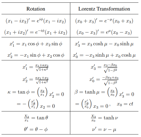
Table 3.1: Summary of the rotational transformations. (The signs of the angles correspond to the passive interpretation.)

Figure 3.1: Area in \(\left(x_{0}, x_{3}\right)\) -plane.

We shall refer to \(\mu\) also as hyperbolic angle. The formal analogy with the circular angle \(\phi\) is evident from the Table. We deepen this parallel by means of the observation that \(\mu\) can be interpreted as an area in the \(\left(x_{0}, x_{3}\right)\) plane (see Figure 3.1).

Consider a hyperbola with the equation

\[\left(\frac{x_{0}}{a}\right)^{2}-\left(\frac{x_{3}}{b}\right)^{2}=1\label{12}\]

\[x_{0}=a \cosh \mu \quad x_{3}=b \sinh \mu\label{13}\]

The shaded triangular area (shown in Figure 3.1) is according to Equation 2.6.2 of Section 2.6:

\[\frac{1}{2}\left|\begin{array}{ll}
x_{3}+d x_{3} & x_{3} \\
x_{0}+d x_{0} & x_{0}
\end{array}\right|=\frac{1}{2}\left(x_{0} d x_{3}-x_{3} d x_{0}\right)=\label{14}\]

\[\frac{a b}{2}\left(\cosh \mu^{2}-\sinh \mu^{2}\right) d=\frac{a b}{2} d \mu\label{15}\]

We could proceed similarly for the circular angle \(\phi\) and define it in terms of the area of a circular sector, rather than an arc. However, only the area can be generalized for the hyperbola.

Although the formulas in Table 3.1 apply also to the wave vector and the four momentum.and can be used in each case also according to the active interpretation, the various situations have their individual features, some of which will now be surveyed.

Consider at first a plane wave the direction of propagation of which makes an angle \(\theta\) with the direction \(x_{3}\) of the Lorentz transformation. We write the phase, Equation \ref{11} of Section 3.2, as

\[\frac{1}{2}\left[\left(k_{0}+k_{3}\right)\left(x_{0}-x_{3}\right)+\left(k_{0}-k_{3}\right)\left(x_{0}+x_{3}\right)\right]-k_{1} x_{1}-k_{2} x_{2}\label{16}\]

This expression is invariant if \(\left(k_{0} \pm k_{3}\right)\) transforms by the same factor \(\exp (\pm \mu) \text { as }\left(x_{0} \pm x_{3}\right)\).

Thus we have

\[k_{3}^{\prime}=k_{3} \cosh \mu-k_{0} \sinh \mu\label{17}\]

\[k_{0}^{\prime}=-k_{3} \sinh \mu+k_{0} \cosh \mu\label{18}\]

Since \(\left(k_{0}, \vec{k}\right)\) is a null-vector, i.e., k has vanishing length, we set

\[k_{3}=k_{0} \cos \theta, \quad k_{3}^{\prime}=k_{0}^{\prime} \cos \theta^{\prime}\label{19}\]

and we obtain for the aberration and the Doppler effect:

\[\cos \theta^{\prime}=\frac{\cos \theta \cosh \mu-\sinh \mu}{\cosh \mu-\cos \theta \sinh \mu}=\frac{\cos \theta-\beta}{1-\beta \cos \theta}\label{20}\]

and

\[\frac{k_{0}^{\prime}}{k_{0}}=\frac{\omega_{0}^{\prime}}{\omega_{0}}=\cosh \mu-\cos \theta \sinh \mu\label{21}\]

For \(\cos \theta=1\) we have

\[\frac{\omega_{0}^{\prime}}{\omega_{0}}=\exp (-\mu)=\sqrt{\frac{1-\beta}{1+\beta}}\label{22}\]

Thus the hyperbolic angle is directly connected with the frequency scaling in the Doppler effect.

Next, we turn to the transformation of the four-momentum of a massive particle. The new feature is that such a particle can be brought to rest. Let us say the particle is at rest in the frame \(\Sigma^{\prime}\) (rest frame), that moves with the velocity \(v_{3}=c \tanh ^{-1} \mu\) in the frame \(\Sigma\) (lab frame). Thus \(v_{3}\) can be identified as the particle velocity along \(x_{3}\).

Solving for the momentum in \(\Sigma^{\prime}\):

\[p_{3}=p_{3}^{\prime} \cosh \mu+p_{0}^{\prime} \sinh \mu\label{23}\]

\[p_{0}=p_{3}^{\prime} \sinh \mu+p_{0}^{\prime} \cosh \mu\label{24}\]

with \(p_{3}^{\prime}=0, p_{0}^{\prime}=m c\), we have

\[p_{3}=m c \sinh \mu=\frac{m c \beta}{\sqrt{1-\beta^{2}}}\label{25}\]

\[p_{0}=m c \cosh \mu=\frac{m c}{\sqrt{1-\beta^{2}}}=\frac{E}{c}\]

\[\gamma=\cosh \mu, \quad \gamma \beta=\sinh \mu\label{26}\]

Thus we have solved the problem posed at the end of Section 3.2.

The point in the preceding argument is that we achieve the transition from a state of rest of a particle to a state of motion, by the kinematic means of inertial transformation. Evidently, the same effect can be achieved by means of acceleration due to a force, and consider this “boost” as an active Lorentz transformation. Let us assume that the particle carries the charge \(e\) and is exposed to a constant electric intensity E. We get from Equantion \ref{25} for small velocities:

\[\frac{d p_{3}}{d t}=m c \cosh \mu \frac{d \mu}{d t} \simeq m c \frac{d \mu}{d t}\label{27}\]

and this agrees with the classical equation of motion if

\[E=\frac{m c}{e} \frac{d \mu}{d t}\label{28}\]

Thus the electric intensity is proportional to the hyperbolic angular velocity.

In close analogy, a circular motion can be produced by a magnetic field:

\[B=-\frac{m c}{e} \frac{d \phi}{d t}=-\frac{m c}{e} \omega\label{29}\]

This is the well known cyclotron relation.

The foregoing results are noteworthy for a number of reasons. They suggest a close connection between electrodynamics and the Lorentz group and indicate how the group theoretical method provides us with results usually obtained by equations of motion.

All this brings us a step closer to our program of establishing much of physics within a group theoretical framework, starting in particular with the Lorentz group. However, in order to carry out this program we have to generalize our technique to three spatial dimensions. For this we have the choice between two methods.

The first is to represent a four-vector as a \(4 × 1\) column matrix and operate on it by \(4 × 4\) matrices involving 16 real parameters among which there are ten relations (see Section 2.5).

The second approach is to map four-vectors on Hermitian \(2 × 2\) matrices

\[P=\left(\begin{array}{cc}
p_{0}+p_{3} & p_{1}-i p_{2} \\
p_{1}+i p_{2} & p_{0}-p_{3}
\end{array}\right)\label{30}\]

and represent Lorentz transformations as

\[P^{\prime}=V P V^{\dagger}\label{31}\]

where \(V \text { and } V^{\dagger}\) are Hermitian adjoint unimodular matrices depending .just on the needed six parameters.

We choose the second alternative and we shall show that the mathematical parameters have the desired simple physical interpretations. In particular we shall arrive at generalizations of the de Moivre relation, Equation \ref{7}.

The balance of this chapter is devoted to the mathematical theory of the \(2×2\) matrices with physical applications to electrodynamics following in Section 4.