3.4: The Pauli Algebra

3.4.1 Introduction

Let us consider the set of all \(2 × 2\) matrices with complex elements. The usual definitions of matrix addition and scalar multiplication by complex numbers establish this set as a four-dimensional vector space over the field of complex numbers \(\mathcal{V}(4, C)\) With ordinary matrix multiplication, the vector space becomes, what is called an algebra, in the technical sense explained at the end of Section 2.3. The nature of matrix multiplication ensures that this algebra, to be denoted \(\mathcal{A}_{2}\) is associative and noncommutative, properties which are in line with the group-theoretical applications we have in mind.

The name “Pauli algebra” stems, of course, from the fact that \(\mathcal{A}_{2}\) was first introduced into physics by Pauli, to fit the electron spin into the formalism of quantum mechanics. Since that time the application of this technique has spread into most branches of physics.

From the point of view of mathematics, \(\mathcal{A}_{2}\) is merely a special case of the algebra \(\mathcal{A}_{n} \text { of } n \times n\) matrices, whereby the latter are interpreted as transformations over a vector space \(\mathcal{V}\left(n^{2}, C\right)\). Their reduction to canonical forms is a beautiful part of modern linear algebra.

Whereas the mathematicians do not give special attention to the case \(n=2\) the physicists, dealing with four-dimensional space-time, have every reason to do so, and it turns out to be most rewarding to develop procedures and proofs for the special case rather than refer to the general mathematical theorems. The technique for such a program has been developed some years ago.

The resulting formalism is closely related to the algebra of complex quaternions, and has been called accordingly a system of hypercomplex numbers. The study of the latter goes back to Hamilton, but the idea has been considerably developed in recent years. The suggestion that the matrices (1) are to be considered symbolically as generalizations of complex numbers which still retain “number-like” properties, is appealing, and we shall make occasional use of it. Yet it seems confining to make this into the central guiding principle. The use of matrices harmonizes better with the usual practice of physics and mathematics.

In the forthcoming systematic development of this program we shall evidently cover much ground that is well known, although some of the proofs and concepts of Whitney and Tisza do not seem to be used elsewhere. However, the main distinctive feature of the present approach is that we do not apply the formalism to physical theories assumed to be given, but develop the geometrical, kinematic and dynamic applications in close parallel with the building up of the formalism.

Since our discussion is meant to be self-contained and economical, we use references only sparingly. However, at a later stage we shall state whatever is necessary to ease the reading of the literature.

3.4.2 Basic Definitions and Procedures

We consider the set \(A_{2} \text { of all } 2 \times 2\) complex matrices

\[A=\left(\begin{array}{ll}
a_{11} & a_{12} \\
a_{21} & a_{22}
\end{array}\right)\label{1}\]

Although one can generate \(\mathcal{A}_{2}\) from the basis

\[e_{1}=\left(\begin{array}{ll}
1 & 0 \\
0 & 0
\end{array}\right)\label{2}\]

\[e_{2}=\left(\begin{array}{ll}
0 & 1 \\
0 & 0
\end{array}\right)\label{3}\]

\[e_{3}=\left(\begin{array}{ll}
0 & 0 \\
1 & 0
\end{array}\right)\label{4}\]

\[e_{4}=\left(\begin{array}{ll}
0 & 0 \\
0 & 1
\end{array}\right)\label{5}\]

in which case the matrix elements are the expansion coefficients, it is often more convenient to generate it from a basis formed by the Pauli matrices augmented by the unit matrix.

Accordingly \(\mathcal{A}_{2}\) is called the Pauli algebra. The basis matrices are

\[\sigma_{0}=I=\left(\begin{array}{ll}
1 & 0 \\
0 & 1
\end{array}\right)\label{6}\]

\[\sigma_{1}=\left(\begin{array}{ll}
0 & 1 \\
1 & 0
\end{array}\right)\label{7}\]

\[\sigma_{2}=\left(\begin{array}{cc}
0 & -i \\
i & 0
\end{array}\right)\label{8}\]

\[\sigma_{3}=\left(\begin{array}{cc}
1 & 0 \\
0 & -1
\end{array}\right)\label{9}\]

The three Pauli matrices satisfy the well known multiplication rules

\[\sigma_{j}^{2}=1 \quad j=1,2,3\label{10}\]

\[\sigma_{j} \sigma_{k}=-\sigma_{k} \sigma_{j}=i \sigma_{l} \quad j k l=123 \text { or an even permutation thereof }\label{11}\]

All of the basis matrices are Hermitian, or self-adjoint:

\[\sigma_{\mu}^{\dagger}=\sigma_{\mu} \quad \mu=0,1,2,3\label{12}\]

(By convention, Roman and Greek indices will run from one to three and from zero to three, respectively.)

We shall represent the matrix A of Equation \ref{1} as a linear combination of the basis matrices with the coefficient of \(\sigma_{\mu}\) denoted by \(a_{\mu}\). We shall refer to the numbers \(a_{\mu}\) as the components of the matrix A. As can be inferred from the multiplication rules, Equation \ref{11} , matrix components are obtained from matrix elements by means of the relation

\[a_{\mu}=\frac{1}{2} \operatorname{Tr}\left(A \sigma_{\mu}\right)\label{13}\]

where Tr stands for trace. In detail,

\[a_{0}=\frac{1}{2}\left(a_{11}+a_{22}\right)\label{14}\]

\[a_{1}=\frac{1}{2}\left(a_{12}+a_{21}\right)\label{15}\]

\[a_{2}=\frac{1}{2}\left(a_{12}-a_{21}\right)\label{16}\]

\[a_{3}=\frac{1}{2}\left(a_{11}-a_{22}\right)\label{17}\]

In practical applications we shall often see that a matrix is best represented in one context by its components, but in another by its elements. It is convenient to have full flexibility to choose at will between the two. A set of four components \(a_{\mu}\), denoted by \(\left\{a_{\mu}\right\}\), will often be broken into a complex scalar \(a_{0}\) and a complex “vector” \(\left\{a_{1}, a_{2}, a_{3}\right\}=\vec{a}\). Similarly, the basis matrices of \(\mathcal{A}_{2}\) will be denoted by \(\sigma_{0}=1 \text { and }\left\{\sigma_{1}, \sigma_{2}, \sigma_{3}\right\}=\vec{\sigma}\). With this notation,

\[A=\sum_{\mu} a_{\mu} \sigma_{\mu}=a_{0} 1+\vec{a} \cdot \vec{\sigma}\label{18}\]

\[=\left(\begin{array}{cc}
a_{0}+a_{3} & a_{1}-i a_{2} \\
a_{1}+i a_{2} & a_{0}-a_{3}
\end{array}\right)\label{19}\]

We associate with .each matrix the half trace and the determinant

\[\frac{1}{2} \operatorname{Tr} A=a_{0}\label{20}\]

\[|A|=a_{0}^{2}-\vec{a}^{2}\label{21}\]

The extent to which these numbers specify the properties of the matrix A, will be apparent from the discussion of their invariance properties in the next two subsections. The positive square root of the determinant is in a way the norm of the matrix. Its nonvanishing: \(|A| \neq 0\) is the criterion for A to be invertible.

Such matrices can be normalized to become unimodular:

\[A \rightarrow|A|^{-1 / 2} A\label{22}\]

The case of singular matrices

\[|A|=a_{0}^{2}-\vec{a}^{2}=0\label{23}\]

calls for comment. We call matrices for which \(|A|=0, \text { but } A \neq 0\), null-matrices. Because of their occurrence, \(\mathcal{A}_{2}\) is not a division algebra. This is in contrast, say, with the set of real quaternions which is a division algebra, since the norm vanishes only for the vanishing quaternion.

The fact that null-matrices are important,stems partly from the indefinite Minkowski metric. However, entirely different applications will be considered later.

We list now some practical rules for operations in \(\mathcal{A}_{2}\), presenting them in terms of matrix components rather than the more familiar matrix elements.

To perform matrix multiplications we shall make use of a formula implied by the multiplication rules, Equation \ref{11}:

\[(\vec{a} \cdot \vec{\sigma})(\vec{b} \cdot \vec{\sigma})=\vec{a} \cdot \vec{b} I+i(\vec{a} \times \vec{b}) \cdot \vec{\sigma}\label{24}\]

where \(\vec{a} \text { and } \vec{b}\) are complex vectors.

Evidently, for any two matrices A and B

\[[A, B]=A B-B A=2 i(\vec{a} \times \vec{b}) \cdot \vec{\sigma}\label{25}\]

The matrices A and B commute, if and only if

\[\vec{a} \times \vec{b}=0\label{26}\]

that is, if the vector parts \(\vec{a} \text { and } \vec{b}\) are “parallel” or at least one of them vanishes.

In addition to the internal operations of addition and multiplication, there are external operations on \(\mathcal{A}_{2}\) as a whole, which are analogous to complex conjugation. The latter operation is an involution, which means that \(\left(z^{*}\right)^{*}=z\). Of the three involutions any two can be considered independent.

In \(\mathcal{A}_{2}\) we have two independent involutions which can be applied jointly to yield a third:

\[A \rightarrow A=a_{0} I+\vec{a} \cdot \vec{\sigma}\label{27}\]

\[A \rightarrow A^{\dagger}=a_{0}^{*} I+\vec{a}^{*} \cdot \vec{\sigma}\label{28}\]

\[A \rightarrow \tilde{A}=a_{0} I-\vec{a} \cdot \vec{\sigma}\label{29}\]

\[A \rightarrow \tilde{A}^{\dagger}=\bar{A}=a_{0}^{*} I-\vec{a}^{*} \cdot \vec{\sigma}\label{30}\]

The matrix \(A^{\dagger}\) is the Hermitian adjoint of A. Unfortunately, there is neither an agreed symbol, nor a term for \(\tilde{A}\) Whitney called it Pauli conjugate, other terms are quaternionic conjugate or hyper-conjugate \(A^{\dagger}\) (see Edwards, l.c.). Finally \(\bar{A}\) is called complex reflection.

It is easy to verify the rules

\[(A B)^{\dagger}=B^{\dagger} A^{\dagger}\label{31}\]

\[(\tilde{A B})=\tilde{B} \tilde{A}\label{32}\]

\[(\overline{A B})=\bar{B} \bar{A}\label{33}\]

According to Equation \ref{33} the operation of complex reflection maintains the product relation in \(\mathcal{A}_{2}\) it is an automorphism. In contrast, the Hermitian and Pauli conjugations are anti-automorphic.

It is noteworthy that the three operations \(\sim, t,-\), together with the identity operator, form a group (the four-group, “Vierergruppe”). This is a mark of closure: we presumably left out no important operator on the algebra.

In various contexts any of the three conjugations appears as a generalization of ordinary complex conjugation.

Here are a few applications of the conjugation rules.

\[A \tilde{A}=\left(a_{0}^{2}-\vec{a}^{2}\right) 1=|A| 1\label{34}\]

For invertible matrices

\[A^{-1}=\frac{\tilde{A}}{|A|}\label{35}\]

For unimodular matrices we have the useful rule:

\[A^{-1}=\tilde{A}\label{36}\]

A Hermitian marrix \(A=A^{\dagger}\) has real components \(h_{0}, \vec{h}\). We define a matrix to be positive if it is Hermitian and has a positive trace and determinant:

\[h_{0}>0, \quad|H|=\left(h_{0}^{2}-\vec{h}^{2}\right)>0\label{37}\]

If H is positive and unimodular, it can be parametrized as

\[H=\cosh (\mu / 2) 1+\sinh (\mu / 2) \hat{h} \cdot \vec{\sigma}=\exp \{(\mu / 2) \hat{h} \cdot \vec{\sigma}\}\label{38}\]

The matrix exponential is defined by a power series that reduces to the trigonometric expression. The factor 1/2 appears only for convenience in the next subsection.

In the Pauli algebra, the usual definition \(U^{\dagger}=U^{-1}\) for a unitary matrix takes the form

\[u_{0}^{*} 1+\vec{u}^{*} \cdot \vec{\sigma}=|U|^{-1}\left(u_{0} 1-\vec{u} \cdot \vec{\sigma}\right)\label{39}\]

If U is also unimodular, then

\[u_{0}^{*}=u_{0}=\text { real }\label{40}\]

\[\vec{u}^{*}=\vec{u}=\text { imaginary }\label{41}\]

and

\[u_{0}^{2}-\vec{u} \cdot \vec{u}=u_{0}^{2}+\vec{u} \cdot \vec{u}^{*}=1\]

\[U=\cos (\phi / 2) 1-i \sin (\phi / 2) \hat{u} \cdot \vec{\sigma}=\exp (-i(\phi / 2) \hat{u} \cdot \vec{\sigma})\label{42}\]

A unitary unimodular matrix can be represented also in terms of elements

\[U=\left(\begin{array}{cc}
\xi_{0} & -\xi_{1}^{*} \\
\xi_{1} & \xi_{0}^{*}
\end{array}\right)\label{43}\]

with

\[\left|\xi_{0}\right|^{2}+\left|\xi_{1}\right|^{2}=1\label{44}\]

where \(\xi_{0}, \xi_{1}\) are the so-called Cayley-Klein parameters. We shall see that both this form, and the axis-angle representation, Equation \ref{42}, are useful in the proper context.

We turn now to the category of normal matrices \(N\) defined by the condition that they commute with their Hermitian adjoint: \(N^{\dagger} N=N N^{\dagger}\) Invoking the condition, Equation \ref{26} , we have

\[\vec{n} \times \vec{n}^{*}=0\label{45}\]

implying that \(n^{*}\) is proportional to n, that is all the components of \(\vec{n}\) must have the same phase. Normal matrices are thus of the form

\[N=n_{0} 1+n \hat{n} \cdot \vec{\sigma}\label{46}\]

where \(n_{0} \text { and } n\) n are complex constants and \(hatn\) is a real unit vector, which we call the axis of N. In particular, any unimodular normal matrix can be expressed as

\[N=\cosh (\kappa / 2) 1+\sinh (\kappa / 2) \hat{n} \cdot \vec{\sigma}=\exp ((\kappa / 2) \hat{n} \cdot \vec{\sigma})\label{47}\]

where \(\kappa=\mu-i \phi,-\infty<\mu<\infty, 0 \leq \phi<4 \pi\), and \(\hat{n}\) is a real unit vector. If \(\hat{n} \text { points in the } " 3 "\) direction, we have

\[N_{0}=\exp \left[\left(\frac{\kappa}{2}\right) \sigma_{3}\right]=\left(\begin{array}{cc}
\exp \left(\frac{\kappa}{2}\right) & 0 \\
0 & \exp \left(-\frac{\kappa}{2}\right)
\end{array}\right)\label{48}\]

Thus the matrix exponentials, Equations \ref{38}, \ref{42} and \ref{48}, are generalizations of a diagonal matrix and the latter is distinguished by the requirement that the axis points in the z direction.

Clearly the normal matrix, Equation \ref{48}, is a commuting product of a positive matrix like Equation \ref{38} with \(\hat{h}=\hat{n}\) and a unitary matrix like Equation \ref{42}, with \(\hat{u}=\hat{n}\)

\[N=H U=U H\label{49}\]

The expressions in Equation \ref{49} are called the polar forms of \(N\), the name being chosen to suggest that the representation of \(N\) by \(H\) and \(U\) is analogous to the representation of a complex number \(z\) by a positive number \(r\) and a phase factor:

\[z=r \exp (-i \phi / 2)\label{50}\]

We shall show that, more generally, any invertible matrix has two unique polar forms

\[A=H U=U H^{\prime}\label{51}\]

but only the polar forms of normal matrices display the following equivalent special features:

1. \(H\) and \(U\) commute

2. \(\hat{h}=\hat{u}=\hat{n}\)

3. \(H^{\prime}=H\)

We see from the polar decomposition theorem that our emphasis on positive and unitary matrices is justified, since all matrices of \(\mathcal{A}_{2}\) can be produced from such factors. We proceed now to prove the theorem expressed in Equation \ref{51} by means of an explicit construction.

First we form the matrix \(A A^{\dagger}\), which is positive by the criteria \ref{36}:

\[a_{0} a_{0}^{*}+\vec{a} \cdot \vec{a}^{*}>0\label{52}\]

\[|A|\left|A^{\dagger}\right|>0\label{53}\]

Let \(A A^{\dagger}\) be expressed in terms of an axis \(\hat{h}\) and the hyperbolic angle \(\mu\):

\[\begin{aligned}
A A^{\dagger} &=b(\cosh \mu 1+\sinh \mu \hat{h} \cdot \hat{\sigma}) \\
&=b \exp (\mu \hat{h} \cdot \hat{\sigma})
\end{aligned}\label{54}\]

where b is a positive constant. We claim that the Hermitian component of A is the positive square root of \ref{54}

\[H=\left(A A^{\dagger}\right)^{1 / 2}=b^{1 / 2} \exp \left(\frac{\mu}{2} \hat{h} \cdot \hat{\sigma}\right)\label{55}\]

with

\[U=H^{-1} A, \quad A=H U\label{56}\]

That U is indeed unitary is easily verified:

\[U^{\dagger}=A^{\dagger} H^{-1}, \quad U^{-1}=A^{-1} H\label{57}\]

and these expressions are equal by Equation \ref{55}.

From Equation \ref{56} we get

\[A=U\left(U^{-1} H U\right)\]

and

\[A=U H^{\prime} \quad \text { with } \quad H^{\prime}=U^{-1} H U\label{58}\]

It remains to be shown that the polar forms \ref{56} are unique. Suppose indeed, that for a particular A we have two factorizations

\[A=H U=H_{1} U_{1}\label{59}\]

then

\[A A^{\dagger}=H^{2}=H_{1}^{2}\label{60}\]

But, since \(A A^{\dagger}\) has a unique positive square root, \(H_{1}=H\), and

\[U=H_{1}^{-1} A=H^{-1} A=U \quad \text { q.e.d. }\label{61}\]

Polar forms are well known to exist for any \(n × n\) matrix, although proofs of uniqueness are generally formulated for abstract transformations rather than for matrices, and require that the transformations be invertable.

3.4.3 The restricted Lorentz group

Having completed the classification of the matrices of \(\mathcal{A}_{2}\), we are ready to interpret them as operators and establish a connection with the Lorentz group. The straightforward procedure would be to introduce a 2-dimensional complex vector space \(\mathcal{V}(\in, \mathcal{C})\). By using the familiar bra-ket formalism we write

\[A|\xi\rangle=\left|\xi^{\prime}\right\rangle\label{62}\]

\[A^{\dagger}\langle\xi|=\left\langle\xi^{\prime}\right|\label{63}\]

The two-component complex vectors are commonly called spinors. We shall study their properties in detail in Section 5. The reason for this delay is that the physical interpretation of spinors is a

subtle problem with many ramifications. One is well advised to consider at first situations in which the object to be operated upon can be represented by a 2 × 2 matrix.

The obvious choice is to consider Hermitian matrices, the components of which are interpreted as relativistic four-vectors. The connection between four-vectors and matrices is so close that it is often convenient to use the same symbol for both:

\[A=a_{0} 1+\vec{a} \cdot \vec{\sigma}\label{64}\]

\[A=\left\{a_{0}, \vec{a}\right\}\label{65}\]

We have

\[a_{0}^{2}-\vec{a}^{2}=|A|=\frac{1}{2} \operatorname{Tr}(A \bar{A})\label{66}\]

or more generally

\[a_{0} b_{0}-\vec{a} \cdot \vec{b}=\frac{1}{2} \operatorname{Tr}(A \bar{B})\label{67}\]

A Lorentz transformation is defined as a linear transformation

\[\left\{a_{0}, \vec{a}\right\}=\mathcal{L}\left\{a_{0}^{\prime}, \vec{a}^{\prime}\right\}\label{68}\]

that leaves the expression \ref{67} and hence also \ref{66} invariant. We require moreover that the sign of the “time component” \(a_{0}\) be invariant (orthochronic Lorentz transformation \(\left.L^{\uparrow}\right)\) and that the determinant of the \(4x4\) matrix \(\mathcal{L}\) be positive (proper Lorentz transformation \(\left.L_{+}\right)\). If both conditions are satisfied, we speak of the restricted Lorentz group \(L_{+}^{\uparrow}\). This is the only one to be of current interest for us, and until further notice “Lorentz group” is to be interpreted in this restricted sense.

Note that A can be interpreted as any of the four-vectors discussed in Section 3.2: \(R=\{r, \vec{r}\}\)

\[K=\left\{k_{0}, \vec{k}\right\}, \quad P=\left\{p_{0}, \vec{p}\right\}\label{69}\]

Although these vectors and their matrix equivalents have identical transformation properties, they differ in the possible range of their determinants. A negative \(|P|\) can arise only for an unphysical imaginary rest mass. By contrast, a positive R corresponds to a time-like displacement pointing toward the future, an R with a negative \(|R|\) to a space-like displacement and \(|R|=0\) is associated with the light cone. For the wave vector we have by definition \(|K|=0\).

To describe a Lorentz transformation in the Pauli algebra we try the “ansatz”

\[A^{\prime}=V A W\label{70}\]

with \(|V|=|W|=1\) in order to preserve \(|A|\). Reality of the vector, i.e., hermiticity of the matrix A is preserved if the additional condition \(W=V^{\dagger}\) is satisfied. Thus the transformation

\[A^{\prime}=V A V^{\dagger}\label{71}\]

leaves expression \ref{66} invariant. It is easy to show that \ref{67} is invariant as well.

The complex reflection \(\bar{A}\) transforms as

\[\overline{A^{\prime}}=\bar{V} \bar{A} \tilde{V}\label{72}\]

and the product of two four-vectors:

\[\begin{aligned}
(A \bar{B})^{\prime} &=V A V^{\dagger} \bar{V} \bar{B} \tilde{V} \\
&=V(A \bar{B}) V^{-1}
\end{aligned}\label{73}\]

This is a so-called similarity transformation. By taking the trace of Equation \ref{73} we confirm that the inner product \ref{67} is invariant under \ref{72}. We have to remember that a cyclic permutation does not affect the trace of a product of matrices. Thus Equation \ref{72} indeed induces a Lorentz transformation in the four-vector space of A.

It is well known that the converse statement is also true: to every transformation of the restricted Lorentz group \(L_{+}^{\uparrow}\) there are associated two matrices differing-only by sign (their parameters \(\phi\) differ by \(2 \pi)\)) in such a fashion as to constitute a two-to-one homomorphism between the group of unimodular matrices \(\mathcal{S L}(2, C)\) and the group \(L_{+}^{\uparrow}\). It is said also that \(\mathcal{S L}(2, C)\) provides a two-valued representation of \(L_{+}^{\uparrow}\). We shall prove this statement by demonstrating explicitly the connection between the matrices V and the induced, or associated group operations.

We note first that \(A \text { and } \bar{A}\) correspond in the tensor language to the contravariant and the covariant representation of a vector. We illustrate the use of the formalism by giving an explicit form for the inverse of \ref{72}

\[A=V^{-1} A^{\prime} V^{\dagger-1} \equiv \tilde{V} A^{\prime} \bar{V}\label{74}\]

We invoke the polar decomposition theorem Equation \ref{49} of Section \ref{2} and note that it is sufficient to establish this connection for unitary and positive matrices respectively.

Consider at first

\[A^{\prime}=U A U^{\dagger} \equiv U A U^{-1}\label{75}\]

with

\[\begin{aligned}
U\left(\hat{u}, \frac{\phi}{2}\right) & \equiv \exp \left(-\frac{i \phi}{2} \hat{u} \cdot \vec{\sigma}\right) \\
u_{1}^{2}+u_{2}^{2}+u_{3}^{2}=1, & 0 \leq \phi<4 \pi
\end{aligned}\label{76}\]

The set of all unitary unimodular matrices described by Equation \ref{76} form a group that is commonly called \(\mathcal{S U}(2)\).

Let us decompose \(\vec{a}:\)

\[\vec{a}=\vec{a}_{\|}+\vec{a}_{\perp}\label{77}\]

\[\vec{a}_{\|}=(\vec{a} \cdot \hat{u}) \hat{u}, \quad \vec{a}_{\perp}=\vec{a}-\vec{a}_{\|}=\hat{u} \times(\vec{a} \times \hat{u})\label{78}\]

It is easy to see that Equation \ref{75} leaves \(a_{0} \text { and } a_{\|}\) invariant and induces a rotation around \(\hat{u}\) by an angle \(\phi: R\{\hat{u}, \phi\}\).

Conversely, to every rotation \(R\{\hat{u}, \phi\}\) there correspond two matrices:

\[U\left(\hat{u}, \frac{\phi}{2}\right) \quad \text { and } \quad U\left(\hat{u}, \frac{\phi+2 \pi}{2}\right)=-U\left(\hat{u}, \frac{\phi}{2}\right)\label{79}\]

We have \(1 \rightarrow 2\) homomorphism between \(\mathcal{S O}(3) \text { and } \mathcal{S} \mathcal{U}(2)\), the latter is said to be a two-valued representation of the former. By establishing this correspondence we have solved the problem of parametrization formulated on page 13. The nine parameters of the orthogonal \(3 × 3\) matrices are reduced to the three independent ones of \(U\left(\hat{u}, \frac{\phi}{2}\right)\). Moreover we have the simple result

\[U^{n}=\exp \left(-\frac{i n \phi}{2} \hat{u} \cdot \vec{\sigma}\right)\label{80}\]

which reduces to the de Moivre theorem if \(\hat{n} \cdot \vec{\sigma}=\sigma_{3}\)

Some comment is in order concerning the two-valuedness of the \(\mathcal{S U}(2)\) representation. This comes about because of the use of half angles in the algebraic formalism which is deeply rooted in the geometrical structure of the rotation group. (See the Rodrigues-Hamilton theorem in Section 2.2.)

Whereas the two-valuedness of the \(\mathcal{S U}(2)\) representation does not affect the transformation of the A vector based on the bilateral expression \ref{75}, the situation will be seen to be different in the spinorial theory based on Equation \ref{62}, since under certain conditions the sign of the spinor \(|\xi\rangle\) is physically meaningful.

The above discussion of the rotation group is incomplete even within the classical theory. The rotation \(R\{\hat{u}, \phi\}\) leaves vectors along \(\hat{u}\) unaffected. A more appropriate object to be rotated is the Cartesian triad, to be discussed in Section 5.

We consider now the case of a positive matrix \(V=H\)

\[A^{\prime}=H A H\label{81}\]

with

\[H=\exp \left(\frac{\mu}{2} \hat{h} \cdot \sigma\right)\label{82}\]

\[h_{1}^{2}+h_{2}^{2}+h_{3}^{2}=1, \quad-\infty<\mu<\infty\label{83}\]

We decompose \(\vec{a}\) as

\[\vec{a}=a \hat{h}+\vec{a}_{\perp}\label{84}\]

and using the fact that \((\vec{a} \cdot \vec{\sigma}) \text { and }(\vec{b} \cdot \vec{\sigma}) \text { commute for } \vec{a} \| \vec{b}\) and anticommute for \(\vec{a} \perp \vec{b}\), we obtain

\[A^{\prime}=\exp \left(\frac{\mu}{2} \hat{h} \cdot \sigma\right)\left(a_{0} 1+a \hat{h} \cdot \sigma+\vec{a}_{\perp} \cdot \sigma\right) \exp \left(\frac{\mu}{2} \hat{h} \cdot \sigma\right)\label{85}\]

\[=\exp (\mu \hat{h} \cdot \sigma)\left(a_{0} 1+\vec{a} \hat{h} \cdot \sigma\right)+\vec{a}_{\perp} \cdot \sigma\label{86}\]

Hence

\[a_{0}^{\prime}=\cosh \mu a_{0}+\sinh \mu a\label{87}\]

\[a^{\prime}=\sinh \mu a_{0}+\cosh \mu a_{0}\label{88}\]

\[\vec{a}_{\perp}^{\prime}=\vec{a}_{\perp}\label{89}\]

This is to be compared with Table 3.1, but remember that we have shifted from the passive to the active interpretation, from alias to alibi.

Positive matrices with a common axis form a group (Wigner’s “little group”), but in general the product of Hermitian matrices with different axes are not Hermitian. There arises a unitary factor, which is the mathematical basis for the famous Thomas precession.

Let us consider now a normal matrix

\[V=N=H\left(\hat{k}, \frac{\mu}{2}\right) U\left(\hat{k}, \frac{\phi}{2}\right)=\exp \left(\frac{\mu-i \phi}{2} \hat{n} \cdot \sigma\right)\label{90}\]

where we have the commuting product of a rotation and a Lorentz transformation with the same axis \(\hat{n}\). Such a constellation is called a Lorentz 4-screw

An arbitrary sequence of pure Lorentz transformations and pure rotations is associated with a pair of matrices \(V\) and \(−V\), which in the general case is of the form

\[H\left(\hat{h}, \frac{\mu}{2}\right) U\left(\hat{u}, \frac{\phi}{2}\right)=U\left(\hat{u}, \frac{\phi}{2}\right) H^{\prime}\left(\hat{h}^{\prime}, \frac{\mu}{2}\right)\label{91}\]

According to Equation \ref{58} of Section \ref{2}, \(H \text { and } H^{\prime}\) are connected by a similarity transformation, which does not affect the angle \(\mu\) but only the axis of the transformation. (See the next section.)

This matrix depends on the 6 parameters, \(\hat{h}, \mu, \hat{u}, \phi\) and thus we have solved the general problem of parametrization mentioned above.

For a normal matrix \(\hat{h}=\hat{u}=\hat{n}\) and the number of parameters is reduced to 4.

Our formalism enables us to give a closed form for two arbitrary normal matrices and the corresponding 4-screws.

\[\left[N, N^{\prime}\right]=2 i \sinh \frac{\kappa}{2} \sinh \frac{\kappa}{2}\left(\hat{n} \times \hat{n}^{\prime}\right) \cdot \vec{\sigma}\label{92}\]

where \(\kappa=\mu-i \phi, \kappa^{\prime}=\mu^{\prime}-i \phi^{\prime}\)

In the literature the commutation relations are usually given in terms of infinitesimal operators which are defined as follows:

\[U\left(\hat{u}_{k}, \frac{d \phi}{2}\right)=1-\frac{i}{2} d \phi \sigma_{k}=1+d \phi I_{k}\label{93}\]

\[I_{k}=-\frac{i}{2} \sigma_{k}\label{94}\]

\[H\left(\hat{h}_{k}, \frac{d \mu}{2}\right)=1+\frac{d \mu}{2} \sigma_{k}=1+d \mu L_{k}\label{95}\]

\[L_{k}=\frac{1}{2} \sigma_{k}\label{96}\]

The commutation relations are

\[\left[I_{1}, I_{2}\right]=I_{3}\label{97}\]

\[\left[L_{1}, L_{2}\right]=-I_{3}\label{98}\]

\[\left[L_{1}, I_{2}\right]=L_{3}\label{99}\]

and cyclic permutations.

It is a well known result of the Lie-Cartan theory of continuous group that these infinitesimalgenerators determine the entire group. Since we have represented these generators in \(\mathcal{S} \mathcal{L}(2, C)\), we have completed the demonstration that the entire group \(L_{+}^{\uparrow}\) is accounted for in our formalism.

3.4.4 Similarity classes and canonical forms of active transformations

It is evident that a Lorentz transformation induced by a matrix \(H\left(\hat{h}, \frac{\mu}{2}\right)\) assumes a particularly simple form if the z-axis of the coordinate system is placed in the direction of \(\hat{h}\). The diagonal matrix \(H\left(\hat{z}, \frac{\mu}{2}\right)\) is said to be the canonical form of the transformation. This statement is a special case of the problem of canonical forms of linear transformations, an important chapter in linear algebra.

Let us consider a linear mapping in a vector space. A particular choice of basis leads to a matrix representation of the mapping, and representations associated with different frames are connected by similarity transformations. Let \(A_{1}\) be an arbitrary and \(S\) an invertible matrix. A similarity transformation is effected on A, by

\[A_{2}=S A_{1} S^{-1}\label{100}\]

Matrices related by similarity transformation are called similar, and matrices similar to each other constitute a similarity class.

In usual practice the mapping-refers to a vector space as in Equation \ref{62} of Section 3.4.3:

\[A_{1}|\xi\rangle_{1}=\left|\xi^{\prime}\right\rangle_{1}\label{101}\]

The subscript refers to the basis “1.” A change of basis \(\Sigma_{1} \rightarrow \Sigma_{2}\) is expressed as

\[|\xi\rangle_{2}=S|\xi\rangle_{1}, \quad\left|\xi^{\prime}\right\rangle_{2}=S\left|\xi^{\prime}\right\rangle_{1}\label{102}\]

Inserting into Equation \ref{101} we obtain

\[A_{1} S^{-1}|\xi\rangle_{2}=S^{-1}|\xi\rangle_{2}\label{103}\]

and hence

\[A_{2}|\xi\rangle_{2}=|\xi\rangle_{2}\label{104}\]

where \(A_{2}\) is indeed given by Equation \ref{100}.

The procedure we have followed thus far to represent Lorentz transformations in \(A_{2}\) does not quite follow this standard pattern.

We have been considering mappings of the space of fourvectors which in turn were represented as 2 × 2 complex matrices. Thus both operators and operands are matrices of \(A_{2}\). In spite of this difference in interpretation, the matrix representations in different frames are still related according to Equation \label{100}.

This can be shown as follows. Consider a unimodular matrix A, that induces a Lorentz transformation in P-space, whereby the matrices refer to the basis \(\Sigma_{1}\):

\[P_{1}^{\prime}=A_{1} P_{1} A_{1}^{\dagger}\label{105}\]

We interpret Equation \ref{105} in the active sense as a linear mapping of P-space on itself that corresponds physically to some dynamic process that alters P in a linear way.

We shall see in Section 4 that the Lorentz force acting on a charged particle during the time dt can be indeed considered as an active Lorentz transformation. (See also page 26.)

The process has a physical meaning independent of the frame of the observer, but the matrix representations of \(P, P^{\prime}\) and of A depend on the frame. The four-momenta in the two frames are connected by a Lorentz transformation interpreted in the passive sense:

\[P_{2}=S P_{1} S^{\dagger}\label{106}\]

\[P_{2}=S P_{1}^{\prime} S^{\dagger}\label{107}\]

with \(|S|=1\). Solving for \(P, P^{\prime}\) and inserting into Equation \ref{105}, we obtain

\[S^{-1} P_{2}^{\prime} \tilde{S}^{\dagger}=A_{1} S^{-1} P_{2} \tilde{S}^{\dagger} A_{1}^{\dagger} S\label{108}\]

or

\[P_{2}^{\prime}=A_{2} P_{2} A_{1}^{\dagger}\label{109}\]

where \(A_{2}\) and \(A_{1}\) are again connected by the similarity transformation \ref{100}.

We may apply the polar decomposition theorem to the matrix S. In the special case that S is unitary, we speak of a unitary similarity transformation corresponding to the rotation of the coordinate system discussed at the onset of this section. However, the general case will lead us to less obvious physical applications.

The above considerations provide sufficient motivation to examine the similarity classes of \(A_{2}\). We shall see that all of them have physical applications, although the interpretation of singular mappings will be discussed only later

The similarity classes can be characterized in several convenient ways. For example, one may use two independent similarity invariants shared by all the matrices \(A=a_{0} l+\vec{a} \cdot \vec{\sigma}\) in the class. We shall find it convenient to choose

1. the determinant |A|, and

2. the quantity \(\vec{a}^{2}\)

The trace is also a similarity invariant, but it is not independent: \(a_{0}^{2}=|A|+\vec{a}^{2}\)

Alternatively, one can characterize the whole class by one representative member of it, some matrix \(A_{0}\) called the canonical form for the class (See Table 3.2).

We proceed at first to characterize the similarity classes in terms of the invariants 1 and 2. We recall that a matrix A is invertible if \(|A| \neq 0\) and singular if \(|A|=0\). Without significant loss of generality, we can normalize the invertible matrices of \(A_{2}\) to be unimodular, so that we need discuss only classes of singular and of unimodular matrices. As a second invariant to characterize a class, we choose \(\vec{a} \cdot \vec{a}\) and we say that a matrix A is axial if \(\vec{a} \cdot \vec{a} \neq 0\). In this case, there exists a unit vector \(\hat{a}\) (possibly complex) such that \(\vec{a}=a \cdot \hat{a}\) where a is a complex constant. The unit vector \(\hat{a}\) is called the axis of A. Conversely, the matrix A is non-axial if \(\vec{a} \cdot \vec{a}=0\), the vector \(\vec{a}\) is called isotropic or a null-vector, it cannot be expressed in terms of an axis.

The concept of axis as here defined is the generalization of the real axis introduced in connection with normal matrices on page 33. The usefulness of this concept is apparent from the following theorem:

Theorem 1. For any two unit vectors \(\hat{v}_{1}, \text { and } \hat{v}_{2}\), real or complex, there exists a matrix S such that

\[\hat{v}_{2} \cdot \vec{\sigma}=S \hat{v}_{1} \cdot \vec{\sigma} S^{1}\label{110}\]

Proof. We construct one such matrix S from the following considerations. If \(\hat{v}_{1}, \text { and } \hat{v}_{2}\) are real, then let S be the unitary matrix that rotates every vector by an angle \(\pi\) about an axis which bisects the angle between \(\hat{v}_{1}, \text { and } \hat{v}_{2}:\)

\[S=-i \hat{s} \cdot \vec{\sigma}\label{111}\]

where

\[\hat{s}=\frac{\hat{v}_{1}+\hat{v}_{2}}{\sqrt{2 \hat{v}_{1} \cdot \hat{v}_{2}+2}}\label{112}\]

Even if \(\hat{v}_{1}, \text { and } \hat{v}_{2}\) are not real, it is easily verified that S as given formally by Equations \ref{111} and \ref{112}, does indeed send \(\hat{v}_{1} \text { to } \hat{v}_{2}\). Naturally S is not unique; for instance, any matrix of the form

\[S=\exp \left\{\left(\frac{\mu_{2}}{2}-i \frac{\phi_{2}}{2}\right) \vec{v}_{2} \cdot \vec{\sigma}\right\}(-i \hat{s} \cdot \vec{\sigma}) \exp \left\{\left(\frac{\mu_{1}}{2}-i \frac{\phi_{1}}{2}\right) \vec{v}_{1} \cdot \vec{\sigma}\right\}\label{113}\]

will send \(\hat{v}_{1} \text { to } \hat{v}_{2}\)

This construction fails only if

\[\hat{v}_{1} \cdot \hat{v}_{2}+1=0\label{114}\]

that is for the transformation \(\hat{v}_{1} \rightarrow-\hat{v}_{2}\). In this trivial case we choose

\[S=-i \hat{s} \cdot \vec{\sigma}, \quad \text { where } \quad \hat{s} \perp \vec{v}_{1}\label{115}\]

Since in the Pauli algebra diagonal matrices are characterized by the fact that their axis is \(\hat{x}_{3}\), we have proved the following theorem:

Theorem 2. All axial matrices are diagonizable, but normal matrices and only normal matrices are diagonizable by a unitary similarity transformation.

The diagonal forms are easily ascertained both for singular and the unimodular cases. (See Table 3.2.) Because of their simplicity they are called also canonical forms. Note that they can be multiplied by any complex number in order to get all of the axial matrices of \(\mathcal{A}_{2}\)

The situation is now entirely clear: the canonical forms show the nature of the mapping; a unitary similarity transformation merely changes the geometrical orientation of the axis. The angle of circular and hyperbolic rotation specified by \(a_{0}\) is invariant. A general transformation complexifies the axis. This situation comes about if in the polar form of the matrix \(A = HU\), the factors have distinct real axes, and hence do not commute.

There remains to deal with the case of nonaxial matrices. Consider \(A=\vec{a} \cdot \vec{\sigma} \text { with } \vec{a}^{2}=0\). Let us decompose the isotropic vector \(\vec{a}\) into real and imaginary parts:

\[\vec{a}=\vec{\alpha}+i \vec{\beta}\label{116}\]

Hence \(\vec{\alpha}^{2}-\vec{\beta}^{2}=0 \text { and } \alpha \cdot \beta=0\). Since the real and the imaginary parts of a are perpendicular, we can rotate these directions by a unitary similarity transformation into the x- and y-directions respectively. The transformed matrix is

\[\frac{\alpha}{2}\left(\sigma_{1}+i \sigma_{2}\right)=\left(\begin{array}{ll}
0 & \alpha \\
0 & 0
\end{array}\right)\label{117}\]

with a positive. A further similarity transformation with

\[S=\left(\begin{array}{cc}
\alpha^{-1 / 2} & 0 \\
0 & \alpha^{1 / 2}
\end{array}\right)\label{118}\]

transforms Equation \ref{117} into the canonical form given in Table 3.2.

As we have seen in Section 3.4.3 all unimodular matrices induce Lorentz transformations in Minkowski, or four-momentum space. According to the results summarized in Table 3.2, the mappings induced by axial matrices can be brought by similarity transformations into so-called Lorentz four-screws consisting of a circular and hyperbolic rotation around the same axis, or in other words: a rotation around an axis, and a boost along the same axis.

What about the Lorentz transformation induced by a nonaxial matrix? The nature of these transformations is very different from the common case, and constitutes an unusual limiting situation. It is justified to call it an exceptional Lorentz transformation. The special status of these transformations was recognized by Wigner in his fundamental paper on the representations of the Lorentz group.

The present approach is much more elementary than Wigner’s, both from the point of view of mathematical technique, and also the purpose in mind. Wigner uses the standard algebraic technique of elementary divisors to establish the canonical Jordan form of matrices. We use, instead a specialized technique adapted to the very simple situation in the Pauli algebra. More important, Wigner was concerned with the problem of representations of the inhomogeneous Lorentz group, whereas we consider the much simpler problem of the group structure itself, mainly in view of application to the electromagnetic theory.

The intuitive meaning of the exceptional transformations is best recognized from the polar form of the generating matrix. This can be carried out by direct application of the method discussed at the end of the last section. It is more instructive, however, to express the solution in terms of (circular and hyperbolic) trigonometry.

We ask for the conditions the polar factors have to satisfy in order that the relation

\[1+\hat{a} \cdot \vec{\sigma}=H\left(\hat{h}, \frac{\mu}{2}\right) U\left(\hat{u}, \frac{\phi}{2}\right)\label{119}\]

should hold with \(\mu \neq 0, \phi \neq 0\). Since all matrices are unimodular, it is sufficient to consider the equality of the traces:

\[\frac{1}{2} \operatorname{Tr} A=\cosh \left(\frac{\mu}{2}\right) \cos \left(\frac{\phi}{2}\right)-i \sinh \left(\frac{\mu}{2}\right) \sin \left(\frac{\phi}{2}\right) \hat{h} \cdot \hat{u}=1\label{120}\]

This condition is satisfied if and only if

\[\hat{h} \cdot \hat{u}=0\label{121}\]

and

\[\cosh \left(\frac{\mu}{2}\right) \cos \left(\frac{\phi}{2}\right)=1\label{122}\]

The axes of circular and hyperbolic rotation are thus perpendicular, to each other and the angles of these rotations are related in a unique fashion: half of the circular angle is the so-called Gudermannian function of half of the hyperbolic angle

\[\frac{\phi}{2}=g d\left(\frac{\mu}{2}\right)\label{123}\]

However, if \(\mu \text { and } \phi\) are infinitesimal, we get

\[\left(1+\frac{\mu^{2}}{2}+\ldots\right)\left(1+\frac{\phi^{2}}{2}+\ldots\right)=1, \text { i.e. }\label{124}\]

\[\mu^{2}-\phi^{2}=0\label{125}\]

We note finally that products of exceptional matrices need not be exceptional, hence exceptional Lorentz transformations do not form a group.

In spite of their special character, the exceptional matrices have interesting physical applications, both in connection with the electromagnetic field as discussed in Section 4, and also for the construction of representations of the inhomogeous Lorentz group [Pae69, Wig39].

We conclude by noting that the canonical forms of Table 3.2 lend themselves to express the powers \(A_{0}^{k}\) in simple form.

For the axial singular matrix we have

\[A_{0}^{2}=A\label{126}\]

These projection matrices are called idempotent. The nonaxial singular matrices are nilpotent:

\[A_{0}^{2}=0\label{127}\]

The exceptional matrices (unimodular nonaxial) are raised to any power k (even non-real) by the formula

\[A^{k}=1^{k}(1+k \vec{a} \cdot \vec{\sigma})\label{128}\]

\[=1^{k} \exp (k \vec{a} \cdot \vec{\sigma})\label{129}\]

For integer k, the factor \(1^{k}\) becomes unity. The axial unimodular case is handled by formulas that are generalizations of the well known de Moivre formulas:

\[A^{k}=1^{k} \exp \left(k \frac{\kappa}{2}+k l 2 \pi i\right)\label{130}\]

where \(l\) is an integer. For integer \(k\), Equation \ref{130} reduces to

\[A^{k}=\exp \left(k\left(\frac{\kappa}{2}\right) \vec{a} \cdot \vec{\sigma}\right)\label{131}\]

In connection with these formulae, we note that for positive \(A(\phi=0\) and a real, there is a unique positive \(\mathrm{m}^{t h}\) root of A:

\[A=\exp \left\{\left(\frac{\mu}{2}\right) \hat{a} \cdot \vec{\sigma}\right\}\label{132}\]

\[A^{1 / m}=\exp \left\{\left(\frac{\mu}{2 m}\right) \hat{a} \cdot \vec{\sigma}\right\}\label{133}\]

The foregoing results are summarized in Table 3.2.

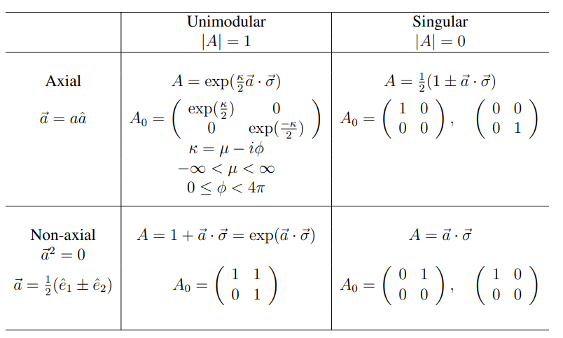
Table 3.2: Canonical Forms for the Simlarity classes of \(A_{2}\)