12.1: The Simplest Markov Chain- The Coin-Flipping Game

Last updated
Save as PDF

Page ID: 34868

\( \newcommand{\vecs}[1]{\overset { \scriptstyle \rightharpoonup} {\mathbf{#1}} } \) \( \newcommand{\vecd}[1]{\overset{-\!-\!\rightharpoonup}{\vphantom{a}\smash {#1}}} \)\(\newcommand{\id}{\mathrm{id}}\) \( \newcommand{\Span}{\mathrm{span}}\) \( \newcommand{\kernel}{\mathrm{null}\,}\) \( \newcommand{\range}{\mathrm{range}\,}\) \( \newcommand{\RealPart}{\mathrm{Re}}\) \( \newcommand{\ImaginaryPart}{\mathrm{Im}}\) \( \newcommand{\Argument}{\mathrm{Arg}}\) \( \newcommand{\norm}[1]{\| #1 \|}\) \( \newcommand{\inner}[2]{\langle #1, #2 \rangle}\) \( \newcommand{\Span}{\mathrm{span}}\) \(\newcommand{\id}{\mathrm{id}}\) \( \newcommand{\Span}{\mathrm{span}}\) \( \newcommand{\kernel}{\mathrm{null}\,}\) \( \newcommand{\range}{\mathrm{range}\,}\) \( \newcommand{\RealPart}{\mathrm{Re}}\) \( \newcommand{\ImaginaryPart}{\mathrm{Im}}\) \( \newcommand{\Argument}{\mathrm{Arg}}\) \( \newcommand{\norm}[1]{\| #1 \|}\) \( \newcommand{\inner}[2]{\langle #1, #2 \rangle}\) \( \newcommand{\Span}{\mathrm{span}}\)\(\newcommand{\AA}{\unicode[.8,0]{x212B}}\)

12.1.1 Game Description

Before giving the general description of a Markov chain, let us study a few specific examples of simple Markov chains. One of the simplest is a "coin-flip" game. Suppose we have a coin which can be in one of two "states": heads (H) or tails (T). At each step, we flip the coin, producing a new state which is H or T with equal probability. In this way, we generate a sequence like "HTTHTHTTHH..." If we run the game again, we would generate another different sequence, like "HTTTTHHTTH..." Each of these sequences is a Markov chain.

This process can be visualized using a "state diagram":

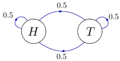
Figure \(\PageIndex{1}\): State diagram for a fair coin-flipping game.

Here, the two circles represent the two possible states of the system, "H" and "T", at any step in the coin-flip game. The arrows indicate the possible states that the system could transition into, during the next step of the game. Attached to each arrow is a number giving the probability of that transition. For example, if we are in the state "H", there are two possible states we could transition into during the next step: "T" (with probability \(0.5\)), or "H" (with probability \(0.5\)). By conservation of probability, the transition probabilities coming out of each state must sum up to one.

Next, suppose the coin-flipping game is unfair. The coin might be heavier on one side, so that it is overall more likely to land on H than T. It might also be slightly more likely to land on the same face that it was flipped from (real coins actually do behave this way). The resulting state diagram can look like this:

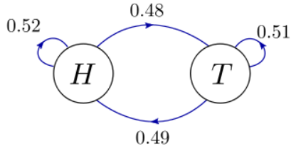
Figure \(\PageIndex{2}\): State diagram for a (particular) unfair coin-flipping game.

Notice that the individual transition probabilities are no longer \(0.5\), reflecting the aforementioned unfair effects. However, the transition probabilities coming out of each state still sum to \(1\) (\(0.52+0.48\) coming out of "H", and \(0.51+0.49\) coming out of "T").

12.1.2 State Probabilities

If we play the above unfair game many times, H and T will tend to occur with slightly different probabilities, not exactly equal to \(0.5\). At a given step, let \(p_{H}\) denote the probability to be in state H, and \(p_{T}\) the probability to be in state T. Let \(P(T|H)\) denote the transition probability for going from H to T, during the next step; and similarly for the other three possible transitions. According to Bayes' rule, we can write the probability to get H on the next step as

\[p_H' = P(H|H) p_H + P(H|T) p_T.\]

Similarly, the probability to get T on the next step is

\[p_T' = P(T|H) p_H + P(T|T) p_T.\]

We can combine these into a single matrix equation:

\[\begin{bmatrix}p_H' \\ p_T'\end{bmatrix} = \begin{bmatrix}P(H|H) & P(H|T) \\ P(T|H) & P(T|T)\end{bmatrix} \begin{bmatrix}p_H \\ p_T\end{bmatrix} = \begin{bmatrix}0.52 & 0.49 \\ 0.48 & 0.51\end{bmatrix} \begin{bmatrix}p_H \\ p_T\end{bmatrix}.\]

The matrix of transition probabilities is called the transition matrix. At the beginning of the game, we can specify the coin state to be (say) H, so that \(p_{H}=1\) and \(p_{T}=0\). If we multiply the vector of state probabilities by the transition matrix, that gives the state probabilities for the next step. Multiplying by the transition matrix \(K\) times gives the state probabilities after \(K\) steps.

After a large number of steps, the states probabilities might converge to a "stationary" distribution, such that they no longer change significantly on subsequent steps. Let these stationary probabilities be denoted by \(\{\pi_H, \pi_T\}\). According to the above equation for transition probabilities, the stationary probabilities must satisfy

\[\begin{bmatrix} \pi_H \\ \pi_T \end{bmatrix} = \begin{bmatrix}P(H|H) & P(H|T) \\ P(T|H) & P(T|T)\end{bmatrix} \begin{bmatrix}\pi_H \\ \pi_T\end{bmatrix}.\]

This system of linear equations can be solved by brute force (we'll discuss a more systematic approach later). The result is

\[\pi_H = \frac{P(H|T)}{P(T|H) + P(H|T)}, \quad \pi_T = \frac{P(T|H)}{P(T|H) + P(H|T)} \qquad (\textrm{stationary}\;\textrm{distribution}).\]

Plugging in the numerical values for the transition probabilities, we end up with \(\pi_H = 0.50515, \; \pi_T = 0.49485\).