12.3: The Ehrenfest Model

12.3.1 Model Description

The coin-flipping game is a "two-state" Markov chain. For physics applications, we're often interested in Markov chains where the number of possible states is huge (e.g. thermodynamic microstates). The Ehrenfest model is a nice and simple example which illustrates many of the properties of such Markov chains. This model was introduced by the husband-and-wife physicist team of Paul and Tatyana Ehrenfest in 1907, in order to study the physics of diffusion.

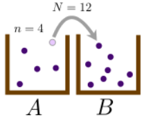
Suppose we have two boxes, labeled A and B, and a total of \(N\) distinguishable particles to distribute between the two boxes. At a given point in time, let there be \(n\) particles in box A, and hence \(N-n\) particles in box B. Now, we repeatedly apply the following procedure:

1. Randomly choose one of the \(N\) particles (with equal probability).
2. With probability \(q\), move the chosen particle from whichever box it happens to be into the other box. Otherwise (with probability \(1-q\)), leave the particle in its current box.

Figure \(\PageIndex{1}\): Schematic of the Ehrenfest model.

If there are \(n\) particles in box A, then we have probability \(n/N\) of choosing a particle in box A, followed by a probability of \(q\) to move that particle into box B. Following similar logic for all the other possibilities, we arrive at three possible outcomes:

• Move a particle from A to B: probability \(nq/N\)
• Move a particle from B to A: probability \((N-n)q/N\)
• Leave the system unchanged: probability \(1-q\)

You can check that (i) the probabilities sum up to \(1\), and (ii) this summary holds true for the end-cases \(n=N\) and \(n=0\).

12.3.2 Markov Chain Description

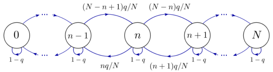
We can label the states of the system using an integer \(n \in \{0, 1, \dots, N\}\), corresponding to the number of particles in box A. There are \(N+1\) possible states, and the state diagram is as follows:

Figure \(\PageIndex{2}\): State diagram for the Ehrenfest model.

Suppose we start out in state \(n_{0}=N\), by putting all the particles in box A. As we repeatedly apply the Ehrenfest procedure, the system goes through a sequence of states, \(\{n_0 = N, n_1, n_2, n_3, \dots\}\), which can be described as a Markov chain. Plotting the state \(n_{k}\) versus the step number \(k\), we see a random trajectory like the one below:

Figure \(\PageIndex{3}\): Sample trajectory of an Ehrenfest model with \(N=50\) and \(q=0.5\).

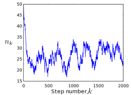
Notice that the system moves rapidly away from its initial state, \(n=50\), and settles into a behavior where it fluctuates around the mid-point state \(n=25\). Let us look for the stationary distribution, in which the probability of being in each state is unchanged on subsequent steps. Let \(\pi_{n}\) denote the stationary probability for being in state \(n\). According to Bayes' rule, this probability distribution needs to satisfy

\[\begin{align} \pi_n &= P(n|n-1) \pi_{n-1} + P(n|n) \pi_n + P(n|n+1) \pi_{n+1} \\ & = \frac{N-n+1}{N} \,q\, \pi_{n-1} + (1-q) \pi_n + \frac{n+1}{N}\,q\, \pi_{n+1}. \end{align}\]

We can figure out \(\pi_{n}\) using two different methods. The first method is to use our knowledge of statistical mechanics. In the stationary distribution, each individual particle should have an equal chance of being in box A or box B. There are \(2^{N}\) possible box assignments, each of which is energetically equivalent and hence have equal probabilities. Hence, the probability of finding \(n\) particles in box A is the number of ways of picking \(n\) particles, which is \(N \choose n\), divided by the number of possible box assignments. This gives

\[\pi_n = {N\choose n} \, 2^{-N}.\]

Substituting into the Bayes' rule formula, we can verify that this distribution is indeed stationary. Note that \(\pi_{n}\) turns out to be independent of \(q\) (the probability of transferring a chosen particle to the other box). Intuitively, \(q\) governs how "quickly" we are transferring particles from one box to the other. Therefore, it should affect how quickly the system reaches its stationary or "equilibrium" behavior, but not the stationary distribution itself.

12.3.3 Detailed Balance

There is another way to figure out \(\pi_{n}\), which doesn't rely on guessing the answer in one shot. Suppose we pick a pair of neighboring states, \(n\) and \(n+1\), and assume that the rate at which the \(n \rightarrow n+1\) transition occurs is the same as the rate at which the opposite transition, \(n \rightarrow n+1\), occurs. Such a condition is not guaranteed to hold, but if it holds for every pair of states, then the probability distribution is necessarily stationary. This situation is called detailed balance. In terms of the state probabilities and transition probabilities, detailed balance requires

\[P(n+1|n) \, \pi_n = P(n|n+1) \, \pi_{n+1} \qquad \forall n \in \{0,\dots,N\},\]

for this Markov chain. Plugging in the transition probabilities, we obtain the recursion relation

\[\pi_{n+1} = \frac{N-n}{n+1}\, \pi_{n}.\]

What's convenient about this recursion relation is that it only involves \(\pi_{n}\) and \(\pi_{n+1}\), unlike the Bayes' rule relation which also included \(\pi_{n-1}\). By induction, we can now easily show that

\[\pi_n = {N\choose n} \pi_0.\]

By conservation of probability, \(\sum_n \pi_n = 1\), we can show that \(\pi_0 = 2^{-N}\). This leads to

\[\pi_n = {N\choose n} 2^{-N},\]

which is the result that we'd previously guessed using purely statistical arguments.

For more complicated Markov chains, it may not be possible to guess the stationary distribution; in such cases, the detailed balance argument is often the best approach. Note, however, that the detailed balance condition is not guaranteed to occur. There are some Markov chains which do not obey detailed balance, so we always need to verify that the detailed balance condition's result is self-consistent (i.e., that it can indeed be obeyed for every pair of states).