13.2: The Ising Model
- Page ID
- 34873

13.2.1 Problem Statement
To better understand the above general formulation of the MCMC method, let us apply it to the 2D Ising model, a simple and instructive model which is commonly used to teach statistical mechanics concepts. The system is described by a set of N "spins", arranged in a 2D square lattice, where the value of each spin \(S_{n}\) is either \(+1\) (spin up) or \(-1\) (spin down). This describes a hypothetical two-dimensional magnetic material, where the magnetization of each atom is constrained to point either up or down.
Each state can be described by a grid of \(+1/=1\) values. For example, for a \(4\times 4\) grid, a typical state can be represented as
\[\begin{align}\{S\} = \left\{\begin{aligned}&+1\: +1\: +1\: -1 \\ &+1\: -1\: -1\: +1 \\ &-1\: +1\: +1\: -1 \\ &-1\: +1 \: -1 \: -1\end{aligned}\right\},\end{align}\]
and the total number of possible states is \(2^{16} = 65536\).
The energy of each state is given by
\[E(\{S\}) = - J \sum_{\langle ij\rangle} S_i S_j,\]
where \(\langle ij\rangle\) denotes pairs of spins, on adjacent sites labeled \(i\) and \(j\), which are adjacent to each other on the grid (without double-counting). We'll assume periodic boundary conditions at the edges of the lattice. Thus, for example,
\[\begin{align}\left\{\begin{aligned}&+1\: +1\: +1\: +1 \\ &+1\: +1\: +1\: +1 \\ &+1 \: +1\: +1\: +1 \\ &+1\: +1\: +1 \: +1\end{aligned}\right\} \quad E = -32J.\end{align}\]
\[\begin{align}\left\{\begin{aligned}&+1\: +1\: -1\: +1 \\ &+1\: +1\: +1\: +1 \\ &+1\: +1\: +1\: +1 \\ &+1\: +1\: +1\: +1\end{aligned}\right\} \quad E = -24J.\end{align}\]
For each state, we can compute various quantities of interest, such as the mean spin
\[S_{\mathrm{avg}}(\{S\}) = \frac{1}{N}\, \sum_i S_i.\]
Here, \(\mathrm{avg}\) denotes the average over the lattice, for a given spin configuration. We are then interested in the thermodynamic average \(\langle S_{\mathrm{avg}}\rangle\), which is obtained by averaging \(S_{\mathrm{avg}}\) over a thermodynamic ensemble of spin configurations:
\[\left\langle S_{\mathrm{avg}}\right\rangle \;\; = \sum_{\mathrm{possible}\;\mathrm{states} \; \{S\}} S_{\mathrm{avg}}(\{S\}) \; \pi(\{S\}),\]
where \(\pi(\{S\})\) denotes the probability of a spin configuration:
\[\pi(\{S\}) = \frac{1}{Z}\, \exp\left(- \frac{E(\{S\})}{kT}\right).\]
13.2.2 Metropolis Monte Carlo Simulation
To apply the MCMC method, we design a Markov process using the Metropolis algorithm discussed above. In the context of the Ising model, the steps are as follows:
- On step \(k\), randomly choose one of the spins, \(i\), and consider a candidate move which consists of flipping that spin: \(S_i \rightarrow -S_i\).
- Calculate the change in energy that would result from flipping spin \(i\), relative to \(kT\), i.e. the quantity:
\[Q \equiv \frac{\Delta E}{kT} = - \left[\frac{J}{kT} \sum_{j\;\mathrm{next}\;\mathrm{to}\;i} S_j\right] \Delta S_i,\]
where \(\Delta S_i\) is the change in \(S_{i}\) due to the spin-flip, which is \(-2\) if \(S_{i}=1\) currently, and \(+2\) if \(S_{i}=-1\) currently. (The reason we calculate \(Q \equiv \Delta E/kT\), rather than \(\Delta E\), is to keep the quantities in our program dimensionless, and to avoid dealing with very large or very small floating-point numbers. Note also that we can do this calculation without summing over the entire lattice; we only need to find the values of the spins adjacent to the spin we are considering flipping.)- If \(Q \le 0\), accept the spin-flip.
- If \(Q>0\), accept the spin-flip with probability \(\exp(-Q)\). Otherwise, reject the flip.
- This tells us the state on step \(k+1\) of the Markov chain (whether the spin was flipped, or remained as it was). Use this to update our moving average of \(S_{\mathrm{avg}}\) (or whatever other average we're interested in).
- Repeat.
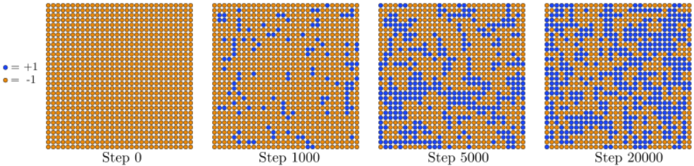
The MCMC method consists of repeatedly applying the above Markov process, starting from some initial state. We can choose either a "perfectly ordered" initial state, where \(S_i = +1\) for all spins, or a "perfectly disordered" state, where each \(S_{i}\) is assigned either \(+1\) or \(-1\) randomly.
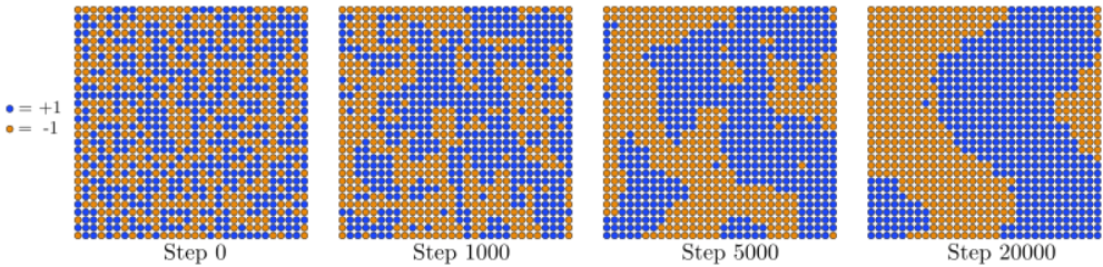
In some systems, the choice of initial state is relatively unimportant; you can choose whatever you want, and leave it to the Markov chain to reach the stationary distribution. For the Ising model, however, there is a practical reason to prefer a "perfectly ordered" initial state, for the following reason. Depending on the value of \(J/kT\), the Ising model either settles into a "ferromagnetic" phase where the spins are mostly aligned, or a "paramagnetic" phase where the spins are mostly random. If the model is in the paramagnetic phase and you start with an ordered (ferromagnetic) initial state, it is easy for the spin lattice to "melt" into disordered states by flipping individual spins, as shown in Figure \(\PageIndex{1}\):
In the ferromagnetic phase, however, if you start with a disordered initial state, the spin lattice will "freeze" by aligning adjacent spins. When this happens, large domains with opposite spins will form, as shown in Figure \(\PageIndex{2}\). These separate domains cannot be easily aligned by flipping individual spins, and as a result the Markov chain gets "trapped" in this part of the state space for a long time, failing to access the more energetically favorable set of states where most of the spins form a single aligned domain. (The simulation will eventually get unstuck, but only if you wait a very long time.) The presence of domains will bias the calculation of \(S_{\mathrm{avg}}\), because the spins in different domains will cancel out. Hence, in this situation is better to start the MCMC simulation in an ordered state.