4.2: Quantum Mechanics in 3D - Angular momentum

Schrödinger equation in spherical coordinates

We now go back to the time-independent Schrödinger equation

\[\left(-\frac{\hbar^{2}}{2 m} \nabla^{2}+V(x, y, z)\right) \psi(x)=E \psi(x) \nonumber\]

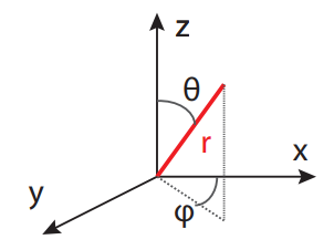
We have already studied some solutions to this equations – for specific potentials in one dimension. Now we want to solve QM problems in 3D. Specifically, we look at 3D problems where the potential \(V(\vec{x}) \) is isotropic, that is, it only depends on the distance from the origin. Then, instead of using cartesian coordinates \(\vec{x}=\{x, y, z\} \), it is convenient to use spherical coordinates \( \vec{x}=\{r, \vartheta, \varphi\}\):

\[ \left\{\begin{array}{l}
x=r \sin \vartheta \cos \varphi \\
y=r \sin \vartheta \sin \varphi \\
x=r \cos \vartheta
\end{array} \Leftrightarrow\left\{\begin{array}{l}
r=\sqrt{x^{2}+y^{2}+z^{2}} \\
\vartheta=\arctan \left(z / \sqrt{x^{2}+y^{2}}\right) \\
\varphi=\arctan (y / x)
\end{array}\right.\right. \nonumber\]

Figure \(\PageIndex{1}\): Spherical Coordinates (CC BY-NC-ND; Paola Cappellaro)

First, we express the Laplacian \( \nabla^{2}\) in spherical coordinates:

\[\nabla^{2}=\frac{1}{r^{2}} \frac{\partial}{\partial r}\left(r^{2} \frac{\partial}{\partial r}\right)+\frac{1}{r^{2} \sin \vartheta} \frac{\partial}{\partial \vartheta}\left(\sin \vartheta \frac{\partial}{\partial \vartheta}\right)+\frac{1}{r^{2} \sin ^{2} \vartheta} \frac{\partial^{2}}{\partial \varphi^{2}} \nonumber\]

To look for solutions, we use again the separation of variable methods, writing \(\psi(\vec{x})=\psi(r, \vartheta, \varphi)=R(r) Y(\vartheta, \varphi) \):

\[-\frac{\hbar^{2}}{2 m}\left[\frac{Y}{r^{2}} \frac{d}{d r}\left(r^{2} \frac{d R}{d r}\right)+\frac{R}{r^{2} \sin \vartheta} \frac{\partial}{\partial \vartheta}\left(\sin \vartheta \frac{\partial Y}{\partial \vartheta}\right)+\frac{R}{r^{2} \sin ^{2} \vartheta} \frac{\partial^{2} Y}{\partial \varphi^{2}}\right]+V(r) R Y=E R Y \nonumber\]

We then divide by RY/r² and rearrange the terms as

\[-\frac{\hbar^{2}}{2 m}\left[\frac{1}{R} \frac{d}{d r}\left(r^{2} \frac{d R}{d r}\right)\right]+r^{2}(V-E)=\frac{\hbar^{2}}{2 m Y}\left[\frac{1}{\sin \vartheta} \frac{\partial}{\partial \vartheta}\left(\sin \vartheta \frac{\partial Y}{\partial \vartheta}\right)+\frac{1}{\sin ^{2} \vartheta} \frac{\partial^{2} Y}{\partial \varphi^{2}}\right] \nonumber\]

Each side is a function of r only and \(\vartheta, \varphi \), so they must be independently equal to a constant C that we set (for reasons to be seen later) equal to \(C=-\frac{\hbar^{2}}{2 m} l(l+1) \). We obtain two equations:

\[\boxed{\frac{1}{R} \frac{d}{d r}\left(r^{2} \frac{d R}{d r}\right)-\frac{2 m r^{2}}{2}(V-E)=l(l+1)} \nonumber\]

and

\[\boxed{\frac{1}{\sin \vartheta} \frac{\partial}{\partial \vartheta}\left(\sin \vartheta \frac{\partial Y}{\partial \vartheta}\right)+\frac{1}{\sin ^{2} \vartheta} \frac{\partial^{2} Y}{\partial \varphi^{2}}=-l(l+1) Y }\nonumber\]

This last equation is the angular equation. Notice that it can be considered an eigenvalue equation for an operator \( \frac{1}{\sin \vartheta} \frac{\partial}{\partial \vartheta}\left(\sin \vartheta \frac{\partial}{\partial \vartheta}\right)+\frac{1}{\sin ^{2} \vartheta} \frac{\partial^{2}}{\partial \varphi^{2}}\). What is the meaning of this operator?

Angular momentum operator

We take one step back and look at the angular momentum operator. From its classical form \(\vec{L}=\vec{r} \times \vec{p} \) we can define the QM operator:

\[\hat{\vec{L}}=\hat{\vec{r}} \times \hat{\vec{p}}=-i \hat{\vec{r}} \times \hat{\vec{\nabla}} \nonumber\]

In cartesian coordinates this reads

\[\begin{array}{l}
\hat{L}_{x}=\hat{y} \hat{p}_{z}-\hat{p}_{y} \hat{z}=-i \hbar\left(y \frac{\partial}{\partial z}-\frac{\partial}{\partial y} z\right) \\
\hat{L}_{y}=\hat{z} \hat{p}_{x}-\hat{p}_{z} \hat{x}=-i \hbar\left(z \frac{\partial}{\partial x}-\frac{\partial}{\partial z} x\right) \\
\hat{L}_{z}=\hat{x} \hat{p}_{y}-\hat{p}_{x} \hat{y}=-i \hbar\left(z \frac{\partial}{\partial y}-\frac{\partial}{\partial x} y\right)
\end{array} \nonumber\]

Some very important properties of this vector operator regard its commutator. Consider for example \(\left[\hat{L}_{x}, \hat{L}_{y}\right] \):

\[\left[\hat{L}_{x}, \hat{L}_{y}\right]=\left[\hat{y} \hat{p}_{z}-\hat{p}_{y} \hat{z}, \hat{z} \hat{p}_{x}-\hat{p}_{z} \hat{x}\right]=\left[\hat{y} \hat{p}_{z}, \hat{z} \hat{p}_{x}\right]-\left[\hat{p}_{y} \hat{z}, \hat{z} \hat{p}_{x}\right]-\left[\hat{y} \hat{p}_{z}, \hat{p}_{z} \hat{x}\right]+\left[\hat{p}_{y} \hat{z}, \hat{p}_{z} \hat{x}\right] \nonumber\]

Now remember that \(\left[x_{i}, x_{j}\right]=\left[p_{i}, p_{j}\right]=0 \) and \(\left[x_{i}, p_{j}\right]=i \delta_{i j} \). Also \( [A B, C]=A[B, C]+[A, C] B\). This simplifies matters a lot

\[\left[\hat{L}_{x}, \hat{L}_{y}\right]=\hat{y}\left[\hat{p}_{z}, \hat{z}\right] \hat{p}_{x}-\cancel{\left[\hat{p}_{y} \hat{z}, \hat{z} \hat{p}_{x}\right]}-\cancel{\left[\hat{y} \hat{p}_{z}, \hat{p}_{z} \bar{x}\right]}+\hat{p}_{y}\left[\hat{z}, \hat{p}_{z}\right] \hat{x}=i \hbar\left(\hat{x} \hat{p}_{y}-\hat{y} \hat{p}_{x}\right)=i \hbar \hat{L}_{z} \nonumber\]

By performing a cyclic permutation of the indexes, we can show that this holds in general:

\[\boxed{\left[\hat{L}_{a}, \hat{L}_{b}\right]=i \hbar \hat{L}_{c}} \nonumber\]

Obs

Since the different components of the angular momentum do not commute, they do not possess common eigenvalues and there is an uncertainty relation for them. If for example I know with absolute precision the angular momentum along the z direction, I cannot have any knowledge of the components along x and y.

Exercise \(\PageIndex{1}\)

What is the uncertainty relation for the x and y components?

\[\Delta L_{x} \Delta L_{y} \geq \frac{\hbar}{2}\left|\left\langle L_{z}\right\rangle\right| \nonumber\]

Exercise \(\PageIndex{2}\)

Assume we know with certainty the angular momentum along the z direction. What is the uncertainty in the angular momentum in the x and y directions?

Answer

From the uncertainty relations, \(\Delta L_{x} \Delta L_{z} \geq \frac{\hbar}{2}\left|\left\langle L_{y}\right\rangle\right|\) and \( \Delta L_{y} \Delta L_{z} \geq \frac{\hbar}{2}\left|\left\langle L_{x}\right\rangle\right|\), we have that if \(\Delta L_{z}=0\) (perfect knowledge) then we have a complete uncertainty in \( L_{x}\) and \(L_{y} \).

Obs.

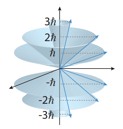
Consider the squared length of the angular momentum vector \( \hat{L}^{2}=\hat{L}_{x}^{2}+\hat{L}_{y}^{2}+\hat{L}_{z}^{2}\). We can show that \(\left[\hat{L}_{a}, \hat{L}^{2}\right]=0 \) (for \(a=\{x, y, z\}\)). Thus we can always know the length of the angular momentum plus one of its components.

For example, choosing the z-component, we can represent the angular momentum as a cone, of length \(\langle L\rangle \), projection on the z-axis \( \left\langle L_{z}\right\rangle\) and with complete uncertainty of its projection along x and y.

We now express the angular momentum using spherical coordinates. This simplifies particularly how the azimuthal angular momentum \(\hat{L}_{z} \) is expressed:

\[ \hat{L}_{x}=i \hbar\left(\sin \varphi \frac{\partial}{\partial \vartheta}+\cot \vartheta \cos \varphi \frac{\partial}{\partial \varphi}\right), \nonumber\]

\[\hat{L}_{y}=-i \hbar\left(\cos \varphi \frac{\partial}{\partial \vartheta}-\cot \vartheta \sin \varphi \frac{\partial}{\partial \varphi}\right), \nonumber\]

\[\hat{L}_{z}=-i \hbar \frac{\partial}{\partial \varphi} \nonumber\]

The form of \( \hat{L}^{2}\) should be familiar:

\[\hat{L}^{2}=-\hbar^{2}\left[\frac{1}{\sin \vartheta} \frac{\partial}{\partial \vartheta}\left(\sin \vartheta \frac{\partial}{\partial \vartheta}\right)+\frac{1}{\sin ^{2} \vartheta} \frac{\partial^{2}}{\partial \varphi^{2}}\right] \nonumber\]

Figure \(\PageIndex{2}\): Graphical representation of the angular momentum, with fixed \(L_{z}\) and L², but complete uncertainty in \(L_{x}\) and \(L_{y}\). (CC BY-NC-ND; Paola Cappellaro)

as you should recognize the angular part of the 3D Schrödinger equation. We can then write the eigenvalue equations for these two operators:

\[\hat{L}^{2} \Phi(\vartheta, \varphi)=\hbar^{2} l(l+1) \Phi(\vartheta, \varphi) \nonumber\]

and

\[\hat{L}_{z} \Phi(\vartheta, \varphi)=\hbar m_{z} \Phi(\vartheta, \varphi) \nonumber\]

where we already used the fact that they share common eigenfunctions (then, we can label these eigenfunctions by \(l\) and \(m_{z}: \Phi_{l, m_{z}}(\vartheta, \varphi)\).

The allowed values for \(l\) and \(m_{z}\) are integers such that \(l=0,1,2, \ldots\) and \(m_{z}=-l, \ldots, l-1, l\). This result can be inferred from the commutation relationship. For interested students, the derivation is below.

Derivation of the eigenvalues. Assume that the eigenvalues of L² and \(L_{z}\) are unknown, and call them \(\lambda\) and \(\mu\). We introduce two new operators, the raising and lowering operators \(L_{+}=L_{x}+i L_{y}\) and \( L_{-}=L_{x}-i L_{y}\). The commutator with \(L_{z} \) is \(\left[L_{z}, L_{\pm}\right]=\pm \hbar L_{\pm}\) (while they of course commute with L²). Now consider the function \(f_{\pm}=L_{\pm} f\), where \(f\) is an eigenfunction of L² and \(L_{z}\):

\[L^{2} f_{\pm}=L_{\pm} L^{2} f=L_{\pm} \lambda f=\lambda f_{\pm} \nonumber\]

and

\[L_{z} f_{\pm}=\left[L_{z}, L_{\pm}\right] f+L_{\pm} L_{z} f=\pm \hbar L_{\pm} f+L_{\pm} \mu f=(\mu \pm \hbar) f_{\pm} \nonumber\]

Then \(f_{\pm}=L_{\pm} f\) is also an eigenfunction of L² and \(L_{z}\). Furthermore, we can keep finding eigenfunctions of \(L_{z}\) with higher and higher eigenvalues \(\mu^{\prime}=\mu+\hbar+\hbar+\ldots\), by applying the \(L_{+}\) operator (or lower and lower with \(L_{-}\)), while the L² eigenvalue is fixed. Of course there is a limit, since we want \(\mu^{\prime} \leq \lambda\). Then there is a maximum eigenfunction such that \(L_{+} f_{M}=0\) and we set the corresponding eigenvalue to \(\hbar l_{M}\). Now notice that we can write L² instead of by using \(L_{x, y}\) by using \( L_{\pm}\):

\[L^{2}=L_{-} L_{+}+L_{z}^{2}+\hbar L_{z} \nonumber\]

Using this relationship on \(f_{M} \) we find:

\[L^{2} f_{m}=\lambda f_{m} \quad \rightarrow \quad\left(L_{-} L_{+}+L_{z}^{2}+\hbar L_{z}\right) f_{M}=\left[0+\hbar^{2} l_{M}^{2}+\hbar\left(\hbar l_{M}\right)\right] f_{M} \quad \rightarrow \quad \lambda=\hbar^{2} l_{M}\left(l_{M}+1\right) \nonumber\]

In the same way, there is also a minimum eigenvalue \( l_{m}\) and eigenfunction s.t. \(L_{-} f_{m}=0 \) and we can find \( \lambda=\hbar^{2} l_{m}\left(l_{m}-1\right)\). Since \( \lambda\) is always the same, we also have \( l_{m}\left(l_{m}-1\right)=l_{M}\left(l_{M}+1\right)\), with solution \(l_{m}=-l_{M} \) (the other solution would have \( l_{m}>l_{M}\)). Finally we have found that the eigenvalues of \( L_{z}\) are between \(+\hbar l \) and \( -\hbar l\) with integer increases, so that \(l=-l+N \) giving \(l\) = N/2: that is, \(l\) is either an integer or an half-integer. We thus set \( \lambda=\hbar^{2} l(l+1)\) and \(\mu=\hbar m, m=-l,-l+1, \ldots, l \). □

We can gather some intuition about the eigenvalues if we solve first the second equation, finding

\[-i \hbar \frac{\partial \Phi_{l, m}}{\partial \varphi}=\hbar m_{z} \Phi(\vartheta, \varphi), \quad \Phi_{l, m}(\vartheta, \varphi)=\Theta_{l}(\vartheta) e^{i m_{z} \varphi} \nonumber\]

where, because of the periodicity in \( \varphi, m_{z}\) can only take on integer values (positive and negative) so that \(\Phi_{l m}(\vartheta, \varphi+2 \pi)=\Phi_{l m}(\vartheta, \varphi)\).

If we solve the first equation, we would find for each eigenvalue \(l\) there are many eigenfunctions. What is the degeneracy of the eigenvalue \(l\)? We know that given \(l, m_{z}\) can take many values (between \(-l\) and \(l\)), in particular 2\(l\) + 1 values. This is the degeneracy of \(l\).

Exercise \(\PageIndex{3}\)

What are the possible values of \(\hat{L}_{x}\) if \(l\) = 7 and \(m_{z}\) = 5?

We know that we can define quantum numbers \(m_{x(y)}\) such that they take integer numbers \(m_{x(y)}=-l, \ldots, l-1, l\). Also, we have the relation among the expectation values:

\[\left\langle\hat{L}^{2}\right\rangle=\left\langle\hat{L}_{x}^{2}+\hat{L}_{y}^{2}+\hat{L}_{z}^{2}\right\rangle \rightarrow l(l+1)=m_{z}^{2}+\left\langle\hat{L}_{x}^{2}+\hat{L}_{y}^{2}\right\rangle / \hbar^{2} \nonumber\]

so in general

\[\left\langle\hat{L}_{x}^{2}\right\rangle \leq \hbar^{2}\left[l(l+1)-m_{z}^{2}\right] \nonumber\]

Then here we have

\[\left\langle\hat{L}_{x}^{2}\right\rangle \leq \hbar^{2}(56-25)=31 \hbar^{2} \nonumber\]

If \( \hat{L}_{x}\) could only take its maximum value (with probability one) we would have \(\left\langle\hat{L}_{x}^{2}\right\rangle=\sum P_{i} L_{x, i}^{2}=L_{x, \max }^{2}\) thus we have \(L_{x, \max } \leq 5 \hbar\) (with 5 the closest integer to \(\sqrt{31}\)). Often, because of symmetry, we have \(\left\langle\hat{L}_{x}^{2}\right\rangle=\left\langle\hat{L}_{y}^{2}\right\rangle\) and,

\[\left\langle\hat{L}_{x}^{2}\right\rangle=\hbar^{2}\left[l(l+1)-m_{z}^{2}\right] \big/ 2 \nonumber\]

thus restricting even further the maximum value of \(L_{x}\).

Spin angular momentum

The quantization of angular momentum gave the result that the angular momentum quantum number was defined by integer values. There is another quantum operator that has the same commutation relationship as the angular momentum but has no classical counterpart and can assume half-integer values. It is called the intrinsic spin angular momentum \(\hat{\vec{S}}\) (or for short, spin). Because it is not a classical properties, we cannot write spin in terms of position and momentum operator. The spin is defined in an abstract spin space (not the usual phase space). Every elementary particle has a specific and immutable value of the intrinsic spin quantum number s (with s determining the eigenvalues of \(\hat{S}^{2}, \hbar^{2} s(s+1)\)), which we call the spin of that particular species: pi mesons have spin 0; electrons have spin 1/2; photons have spin 1; gravitons have spin 2; and so on. By contrast, the orbital angular momentum quantum number \(l\) of a particle can a priori take on any (integer) value, and \(l\) will change when the system is perturbed.

The eigenvectors of the spin operators are not spherical harmonics. Actually, since the spin is not defined in terms of position and momentum, they are not a function of position and are not defined on the usual phase space. The eigenstates are instead described by linear vectors, for example, two-dimensional vectors for the spin-\(\frac{1}{2}\). Thus the operators will be as well represented by matrices.

We already saw the operators describing the spin-\(\frac{1}{2}\) operators and we even calculated their eigenvalues and eigenvec­tors (see section 2.2).

We can then also define the total angular momentum, which is the sum of the usual angular momentum (called the orbital angular momentum) and the spin:

\[\hat{\vec{J}}=\hat{\vec{L}}+\hat{\vec{S}} \nonumber\]

What is the meaning of the sum of two angular momentum operators and what are the eigenvalues and eigenfunctions of the resulting operators?

Addition of angular momentum

We have seen above that any elementary particle posses an intrinsic spin. Then, we can always define the total angular momentum as the sum of the orbital angular momentum and the intrinsic spin. This is an example of addition of angular momentum. Then of course we could also consider two distinct particles and ask what is the total orbital angular momentum of the two particles (or of more particles). There are thus many cases of addition of angular momentum, for example:

1. \(\hat{\vec{J}}=\hat{\vec{L}}+\hat{\vec{S}}\)
2. \(\hat{\vec{L}}=\hat{\vec{L}}_{1}+\hat{\vec{L}}_{2}\)
3. \(\hat{\vec{J}}=\hat{\vec{J}}_{1}+\hat{\vec{J}}_{2}=\hat{\vec{L}}_{1}+\hat{\vec{S}}_{1}+\hat{\vec{L}}_{2}+\hat{\vec{S}}_{2}\)
4. \(\hat{\vec{S}}=\hat{\vec{S}}_{1}+\hat{\vec{S}}_{2}+\hat{\vec{S}}_{3}\)
5. ...

Consider for example the second case. A possible state of the two particles can be described by the eigenvalues/eigenfunctions of each particle angular momentum. For example we could specify \(l_{1}\) and \(m_{z}^{1}\) as well as \(l_{2}\) and \(m_{z}^{2}\) (I will from now on just write \(m_{1}\) and \(m_{z}^{1}\) etc.). Then a state could be for example written in Dirac’s notation as \(\left|l_{1}, m_{1}, l_{2}, m_{2}\right\rangle\). This however does not tell us anything about the total system and its angular momentum. Sometime this quantity is more interesting (for example if the two particles are interacting, their total angular momentum is bound to determine their energy, and not the state of each particle alone).

Coupled and uncoupled representations

The sum of angular momentum satisfy the general commutation rules, \(\left[L^{2}, L_{z}\right]=0,\left[L_{x}, L_{y}\right]=i L_{z}\) etc. We can then also define the eigenvalues (and eigenfunctions) of the total angular momentum \(\hat{\vec{L}}\), for example \(l\) (for L²) and m (for \(L_{z}\)). However, since we only have 2 quantum numbers, we expect the eigenfunctions to be degenerate and we still need to find two more quantum numbers. Equivalently, what we need to do is to find a complete set of commuting observables, such that an eigenfunction (common to all these observables) is well defined –no ambiguity in it– by the set of eigenvalues (or quantum numbers) of the observables.

The first question we can ask is : are these eigenfunctions going to be in common with the single particle operators? To determine this, we need to look at the commutation of the operators.

Now we know that \(\left[L_{1}^{2}, L_{z, 1}\right]=0\), but what about \(\left[L^{2}, L_{z, 1}\right] \)?

We first express L² explicitly: \(L^{2}=\left|\hat{\vec{L}_{1}}+\hat{\bar{L}_{2}}\right|^{2}=L_{1}^{2}+L_{2}^{2}+2 \hat{\vec{L}}_{1} \cdot \hat{\vec{L}}_{2}\). Then the commutator is:

\[\left[L^{2}, L_{z, 1}\right]=\left[L_{1}^{2}+L_{2}^{2}+2\left(L_{x, 1} L_{x, 2}+L_{y, 1} L_{y, 2}+L_{z}^{1} L_{z}^{2}\right), L_{z, 1}\right] \nonumber\]

\[=\left[2\left(L_{x, 1} L_{x, 2}+L_{y, 1} L_{y, 2}\right), L_{z, 1}\right]=2 i\left(\left(L_{y, 1} L_{x, 2}-L_{x, 1} L_{y, 2}\right) \neq 0\right. \nonumber\]

Thus the two operators do not commute and do not share common eigenfunctions. What about \(L_{1}^{2} \)?

\[\left[L^{2}, L_{1}^{2}\right]=\left[L_{1}^{2}+L_{2}^{2}+2\left(L_{x, 1} L_{x, 2}+L_{y, 1} L_{y, 2}+L_{z}^{1} L_{z}^{2}\right), L_{1}^{2}\right]=0 \nonumber\]

since \(\left[L_{1}^{2}, L_{a, 1}\right]=0 \). This means that there are common eigenfunctions of \( L_{1}^{2}, L_{2}^{2}, L^{2}\) and \(L_{z} \). These operators are a complete set of commuting observables. An eigenfunction is thus well defined by the set of eigenvalues \(l, m, l_{1}\) and \(l_{2}\) and we can write the eigenstates as \(\psi_{l, m, l_{\mathrm{i}}, l_{2}}\) or \(\left|l, m, l_{1}, l_{2}\right\rangle\).

There are then two possible representations of the combined system (two possible basis to represent a general state):

\[\begin{array}{lcc}\hline \textbf { Representation } & \textbf { Eigenstates } & \textbf { Complete set of commuting observables } \\ \text { Uncoupled } & \left|l_{1}, m_{1}, l_{2}, m_{2}\right\rangle, & L_{1}^{2}, L_{2}^{2}, L_{1, z} \text { and } L_{2, z} \\ \text { Coupled } & \left|l, m, l_{1}, l_{2}\right\rangle, & L_{1}^{2}, L_{2}^{2}, L^{2} \text { and } L_{z} \\ \hline \end{array} \nonumber\]

How do we go from one basis to the other? As usual this is done by expressing each vector in one basis as a linear combination of vectors in the other basis:

\[\left|l, m, l_{1}, l_{2}\right\rangle=\sum_{m_{1}, m_{2}} c_{m_{1}, m_{2}}^{l}\left|l_{1}, m_{1}, l_{2}, m_{2}\right\rangle \nonumber\]

Notice that since the total angular momentum in the \(z\) direction must be \(m\), we limit the sum to terms s.t. \(m_{1}+m_{2}=m\).

What are the coefficients \(c_{m_{1}, m_{2}}^{l}\)?

Since the two representations are two orthogonal basis, we have that \(\left\langle l_{1}^{\prime}, m_{1}^{\prime}, l_{2}^{\prime}, m_{2}^{\prime} \mid l_{1}, m_{1}, l_{2}, m_{2}\right\rangle=0\) unless all the indexes are equal. Then the coefficient can be calculated (as usual!) from the inner product of \(\left|l_{1}, m_{1}, l_{2}, m_{2}\right\rangle\) and \(\left|l, m, l_{1}, l_{2}\right\rangle\):

\[c_{m_{1}, m_{2}}^{l}=\left\langle l_{1}, m_{1}, l_{2}, m_{2} \mid l, m, l_{1}, l_{2}\right\rangle \nonumber\]

These coefficients are called the Clebsch-Gordon coefficients.

Addition rules: Two particles

In describing the energy levels of atoms and nuclei it is very convenient to be able to find the allowed values of (l, m) given the values of (\(l_{1}, l_{2}\)) for two given particles (e.g. electrons, protons or neutrons). Indeed, we saw that the operator \(\hat{L}^{2}\) appears in the Hamiltonian of the system. Thus its eigenvalue \(\hbar^{2} l(l+1)\) will be important in determining the system energy.

Even if we cannot fix the value of \(l\) if we only know \(l_{1}, m_{1}, l_{2}\) and \(m_{2}\) we can at least restrict the possible values of \(l\). In order to do so, one has to analyze the possible maximum length of the total angular momentum and the degeneracy of the eigenvalues.

1. Maximum \(l\): For two particles with quantum numbers \(l_{1}\) and \(l_{2}\) we know that in the coupled representation we cannot fix the values of \(m_{1}\) and \(m_{2}\). However, we know that given \(l_{1}\) and \(l_{2}\) only some values of \(m_{1}\) and \(m_{2}\) are allowed (e.g. \(m_{1}=-l_{1},-l_{1}+1, \ldots, l_{1}\). Then the maximum values of \(m_{1}\) and \(m_{2}\) are \(m_{1}=l_{1}\) and \(m_{2}=l_{2}\). This also determines the maximum value of \(m: m_{\max }=l_{1}+l_{2}\). But \(m\) itself can only take values \(m=-l, \ldots, l-1, l\).
   Then the maximum value of \(l\) is \(m_{\max }=l_{\max }\).
   Thus, what we just proved is that \(l \leq l_{1}+l_{2}\).
2. Minimum \(l\): To find the minimum \(l\) value we need to look at the degeneracy of the state \(\left|l, m, l_{1}, l_{2}\right\rangle\). Since this state could be also written (in the uncoupled representation) as \(\sum_{m_{1}+m_{2}=m} c_{m_{1}, m_{2}}^{l}\left|l_{1}, m_{1}, l_{2}, m_{2}\right\rangle\), the degeneracy of the state must be the same. What are the two degeneracies?
   We know that for a given angular momentum operator \(\hat{L}\) with total angular momentum quantum number \(l\), there are 2\(l\) + 1 states with the same angular momentum \(\hbar^{2} l(l+1)\).
   Then, considering the uncoupled representation we have \(\mathcal{D}=\left(2 l_{1}+1\right)\left(2 l_{2}+1\right)\) possible states with \(l_{1}\) and \(l_{2}\). In the coupled representation instead we have to consider all the states that have an allowed \(l: \mathcal{D}=\sum_{l=l_{\min }}^{l_{1}+l_{2}}(2 l+1)\). We want these two quantities to be equal. Now remember that \(\sum_{k=1}^{K} k=\frac{K(K+1)}{2}\). Then \(\sum_{l=l_{m i n}}^{l_{1}+l_{2}}(2 l+1)=\left(1+l_{1}+\right.\left.l_{2}\right)^{2}-l_{\min }^{2}\), so that \(l_{\min }^{2}=\left(1+l_{1}+l_{2}\right)^{2}-\left(2 l_{1}+1\right)\left(2 l_{2}+1\right)=\left(l_{1}-l_{2}\right)^{2}\).
   Using the degeneracy condition we thus proved that \(l \geq\left|l_{1}-l_{2}\right|\).

The addition rule states thus that

\[\boxed{\text{The total angular momentum quantum number is bounded by } \left|l_{1}-l_{2}\right| \leq l \leq l_{1}+l_{2} }\nonumber\]

Example \(\PageIndex{1}\)

Consider two spins-1/2 particles (for example two electrons with zero orbital angular momentum). Since we choose spin-\(\frac{1}{2}\) we have only 1 possible value s = \(\frac{1}{2}\) and two values for \(m_{z}: m_{z}=\pm \frac{1}{2}\). We can omit writing explicitly the s quantum number (since it’s always \(\frac{1}{2}\), and we write \(\left|+\frac{1}{2},+\frac{1}{2}\right\rangle=\left|+\frac{1}{2}\right\rangle\) and \(\left|+\frac{1}{2},-\frac{1}{2}\right\rangle=\left|-\frac{1}{2}\right\rangle\). A basis for the uncoupled representation is then given by:

\[\left|s_{1}, m_{1}, s_{2}, m_{2}\right\rangle=\left\{\begin{array}{l}
\left|+\frac{1}{2},+\frac{1}{2},+\frac{1}{2},+\frac{1}{2}\right\rangle=\left|+\frac{1}{2},+\frac{1}{2}\right\rangle \\
\left|+\frac{1}{2},+\frac{1}{2},+\frac{1}{2},-\frac{1}{2}\right\rangle=\left|+\frac{1}{2},-\frac{1}{2}\right\rangle \\
\left|+\frac{1}{2},-\frac{1}{2},+\frac{1}{2},+\frac{1}{2}\right\rangle=\left|-\frac{1}{2},+\frac{1}{2}\right\rangle \\
\left|+\frac{1}{2},-\frac{1}{2},+\frac{1}{2},-\frac{1}{2}\right\rangle=\left|-\frac{1}{2},-\frac{1}{2}\right\rangle
\end{array}\right. \nonumber\]

Consider now the coupled representation. The possible values for s are 1 or 0. In the first case, we have 3 possible values for \(m\) = −1, 0, 1. While the second only has \(m\) = 0. Again, since the values of \(s_{1}\) and \(s_{2}\) are fixed we do not write them:

\[\left|s, m, s_{1}, s_{2}\right\rangle=\left\{\begin{array}{l}
\left.0,0, \frac{1}{2}, \frac{1}{2}\right\rangle=|0,0\rangle \\
\left.1,-1, \frac{1}{2}, \frac{1}{2}\right\rangle=|1,-1\rangle \\
\left.1,0, \frac{1}{2}, \frac{1}{2}\right\rangle=|1,0\rangle \\
\left.1,1, \frac{1}{2}, \frac{1}{2}\right\rangle=|1,1\rangle
\end{array}\right. \nonumber\]

In this particular example it is easy to calculate the Clebsch-Gordon coefficients and we find the relations between the two representations:

\[\begin{array}{ll}
|0,0\rangle= & \frac{\left|+\frac{1}{2},-\frac{1}{2}\right\rangle-\left|-\frac{1}{2},+\frac{1}{2}\right\rangle}{\sqrt{2}} \\
|1,-1\rangle= & \left|-\frac{1}{2},-\frac{1}{2}\right\rangle \\
|1,0\rangle= & \frac{\left|+\frac{1}{2},-\frac{1}{2}\right\rangle+\left|-\frac{1}{2},+\frac{1}{2}\right\rangle}{\sqrt{2}} \\
|1,1\rangle= & \left|+\frac{1}{2},+\frac{1}{2}\right\rangle
\end{array} \nonumber\]

Addition rules: many particles

The addition rules can be generalized to many particles, by just repetitively applying the two-particle rules. We then find for N particles:

• \(l_{\max }=\sum_{k=1}^{N} l_{k}\)
• \(l_{\min }=\max \left\{0,2 l_{N}-l_{\max }\right\}\)

where \(l_{N}\) is the largest of the \(\left\{l_{k}\right\}\).