8.4: Bose-Einstein and Fermi-Dirac Statistics

Finally, in this section we will derive the Bose-Einstein and Fermi-Dirac statistics. In particular, we are interested in the thermal equilibrium for a large number of (non-interacting) identical particles with some energy spectrum \(E_{j}\), which my be continuous.

Since the number of particles is not fixed, we are dealing with the Grand Canonical Ensemble. Its partition function \(\Xi\) is given by

\[\Xi=\operatorname{Tr}\left[e^{\mu \beta \hat{n}-\beta H}\right],\tag{8.43}\]

where \(H\) is the many-body Hamiltonian, \(\beta=1 / k_{B} T\) and \(\mu\) is the chemical potential. The average number of particles with single particle energy \(\boldsymbol{E}_{j}\) is then given by

\[\left\langle n_{j}\right\rangle=-\frac{1}{\beta} \frac{\partial \ln \Xi}{\partial E_{j}}.\tag{8.44}\]

For the simple case where \(H=\sum_{j} E_{j} \hat{n}_{j}\) and the creation and annihilation operators obey the commutator algebra, the exponent can be written as

\[\exp \left[\beta \sum_{j}\left(\mu-E_{j}\right) \hat{a}_{j}^{\dagger} \hat{a}_{j}\right]=\bigotimes_{j} \sum_{n_{j}=0}^{\infty} e^{\beta\left(\mu-E_{j}\right) n_{j}}\left|n_{j}\right\rangle\left\langle n_{j}\right|,\tag{8.45}\]

and the trace becomes

\[\Xi=\prod_{j} \frac{1}{1-e^{\beta\left(\mu-E_{j}\right)}}.\tag{8.46}\]

The average photon number for energy \(\boldsymbol{E}_{j}\) is

\[\left\langle n_{j}\right\rangle=-\frac{1}{\beta} \frac{\partial \ln \Xi}{\partial E_{j}}=-\frac{1}{\beta \Xi} \frac{\partial \Xi}{\partial E_{j}}=\frac{1}{e^{-\beta\left(\mu-E_{j}\right)}-1}.\tag{8.47}\]

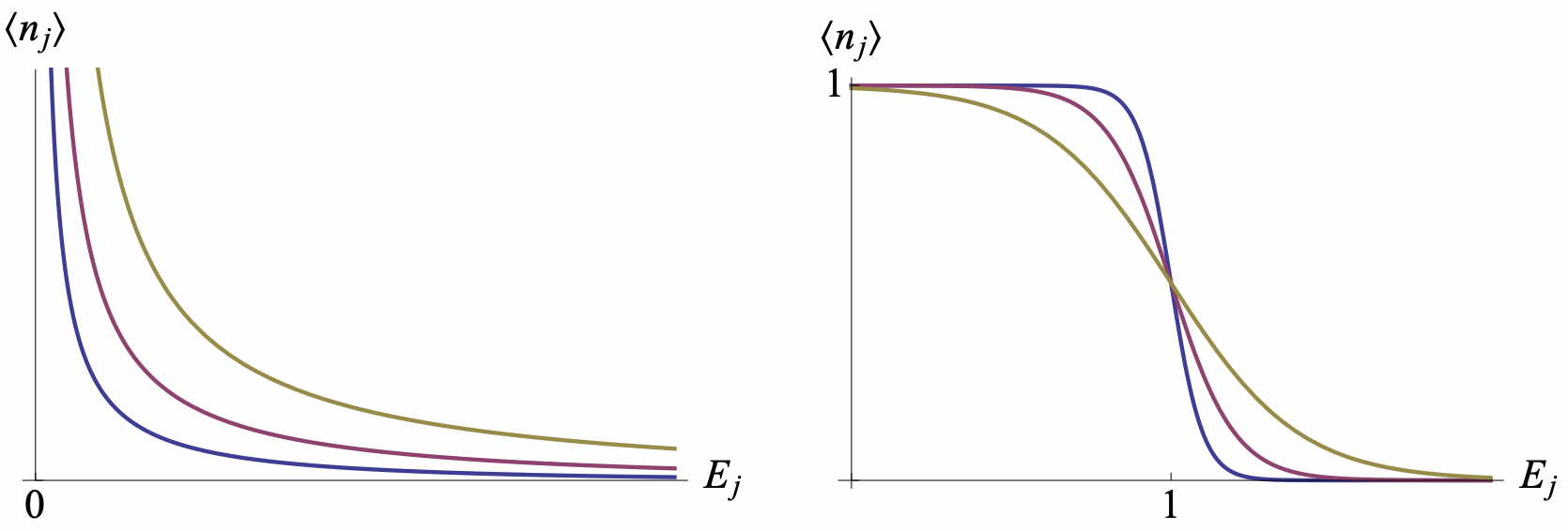
This is the Bose-Einstein distribution for particles with energy \(E_{j}\). It is shown for increasing \(E_{j}\) in Fig. 4 on the left.

Figure 4: Left: Bose-Einstein distribution for different temperatures \((\mu=0)\). The lower the temperature, the more particles occupy the low energy states. Right: Fermi-Dirac distribution for different temperatures and \(\mu=1\). The fermions will not occupy energy states with numbers higher than 1, and therefore higher energies are necessarily populated. The energy values \(E_{j}\) form a continuum on the horizontal axis.

Alternatively, if the creation and annihilation operators obey the anti-commutation relations, the sum over \(n_{j}\) in Eq. (8.45) runs not from 0 to ∞, but over 0 and 1. The partition function of the grand canonical ensemble then becomes

\[\Xi=\prod_{j}\left[1+e^{\beta\left(\mu-E_{j}\right)}\right],\tag{8.48}\]

and the average number of particles with energy \(E_{j}\) becomes

\[\left\langle n_{j}\right\rangle=-\frac{1}{\beta \Xi} \frac{\partial \Xi}{\partial \hbar \omega_{j}}=\frac{1}{e^{-\beta\left(\mu-E_{j}\right)}+1}.\tag{8.49}\]

This is the Fermi-Dirac statistics for these particles, and it is shown in Fig. 4 on the right. The chemical potential is the highest occupied energy at zero temperature, and in solid state physics this is called the Fermi level. Note the sign difference in the denominator with respect to the Bose-Einstein statistics.

Exercises

1. Calculate the Slater determinant for three electrons and show that no two electrons can be in the same state.
2. Particle statistics.
   1. What is the probability of finding \(n\) bosons with energy \(E_{j}\) in a thermal state?
   2. What is the probability of finding \(n\) fermions with energy \(E_{j}\) in a thermal state?
3. Consider a system of (non-interacting) identical bosons with a discrete energy spectrum and a ground state energy \(\boldsymbol{E}_{0}\). Furthermore, the chemical potential starts out lower than the ground state energy \(\mu<E_{0}\).
   1. Calculate \(\left\langle n_{0}\right\rangle\) and increase the chemical potential to \(\mu \rightarrow E_{0}\) (e.g., by lowering the temperature). What happens when \(\mu\) passes \(\boldsymbol{E}_{0}\)?
   2. What is the behaviour of \(\left\langle n_{\text {thermal }}\right\rangle \equiv \sum_{j=1}^{\infty}\left\langle n_{j}\right\rangle\) as \(\mu \rightarrow E_{0}\)? Sketch both \(\left\langle n_{0}\right\rangle\) and \(\left\langle n_{\text {thermal }}\right\rangle\) as a function of \(\mu\). What is the fraction of particles in the ground state at \(\mu=E_{0}\)?
   3. What physical process does this describe?
4. The process \(U=\exp \left(r \hat{a}_{1}^{\dagger} \hat{a}_{2}^{\dagger}-r^{*} \hat{a}_{1} \hat{a}_{2}\right)\) with \(r \in \mathbb{C}\) creates particles in two systems, 1 and 2, when applied to the vacuum state \(|\Psi\rangle=U|\varnothing\rangle\).
   1. Show that the bosonic operators \(\hat{a}_{1}^{\dagger} \hat{a}_{2}^{\dagger}\) and \(\hat{a}_{1} \hat{a}_{2}\) obey the algebra

      \(\left[K_{-}, K_{+}\right]=2 K_{0} \quad \text { and } \quad\left[K_{0}, K_{\pm}\right]=\pm K_{\pm},\)

      with \(K_{+}=K_{-}^{\dagger}\).

   2. For operators obeying the algebra in (a) we can write

      \[\begin{aligned}
      e^{r K_{+}-r^{*} K_{-}}=\exp \left[\frac{r}{|r|} \tanh |r| K_{+}\right] & \exp \left[-2 \ln (\cosh |r|) K_{0}\right] \\
      & \times \exp \left[-\frac{r^{*}}{|r|} \tanh |r| K_{-}\right].
      \end{aligned}\tag{8.50}\]

      Calculate the state \(|\Psi\rangle\) of the two systems.

   3. The amount of entanglement between two systems can be measured by the entropy \(S(r)\) of the reduced density matrix \(\rho_{1}=\operatorname{Tr}_{1}[\rho]\) for one of the systems. Calculate \(S(r)=-\operatorname{Tr}\left[\rho_{1} \ln \rho_{1}\right]\).
   4. What is the probability of finding \(n\) particles in system 1?