14.3.1: s Orbitals

Orbits with \(l = 0\) are called \(s\) orbitals. Although this is not where the letter comes from, it’s useful to think of these as “spherical” orbitals, because they are spherically symmetric. However, they aren’t just spheres! Again, remember that the probability cloud for the electron is a fuzzy ball around the nucleus, representing where the electron is likely to be found.

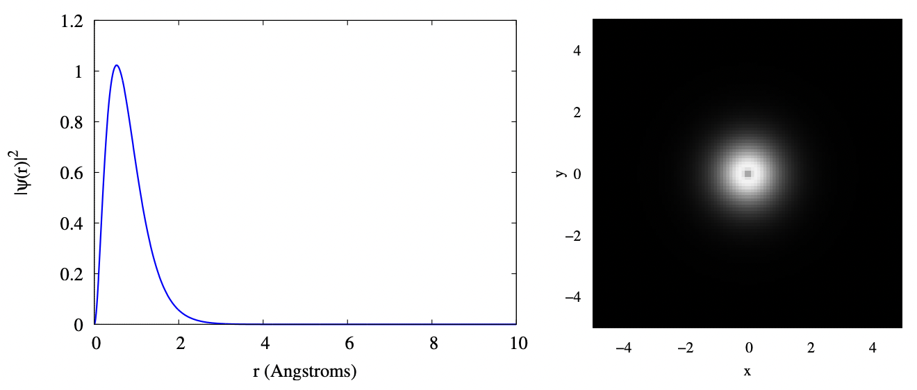
The plot below shows two visualizations of the 1s orbital. On the left is a plot of \(\Psi^{*}(r) \Psi(r)\). This gives the probability density for the electron to be found at radius \(r\). That is, you must pick a small range \(dr\) around the \(r\) you’re interested in, and multiply this probability density by that \(dr\). You then get the probability for finding the electron with that \(dr\) of your chosen \(r\). On the right is a cut through the \(x − z\) plane showing the probability density as a function of position. Lighter colors mean more probability of finding the electron at that position. Notice that there is a darker spot at the center. This corresponds to the probability dropping to zero at \(r = 0\), as seen in the left plot. In both cases, distances are plotted in terms of Angstroms; one Angstrom is 10⁻¹⁰ m which, as you can see from the plot, is about the size of an atom.

If you go to the 2s orbitals, an additional bump is added to the radial wave function. Also, the average distance the electron is from the center of the atom gets larger. While the probability clouds for a 1s and 2s orbital overlap, most of the probability for a 2s electron is outside most of the probability for a 1s electron. This means that to some extent, when working out the properties of an atom with two electrons in the 1s shell and one 2s electron (that would be Lithium), we can treat the nucleus plus the 1s shell as a single spherical ball of net charge +1. While this isn’t perfect, this does lend some support to the approximation we’ll make for multielectron atoms that each electron is moving in a nuclear potential and not interfering too much with other electrons.

Below are the same two plots for the 2s orbital. The scale of the axes is the same as the scale used previously in the 1s orbital, so that you may compare the plots directly.

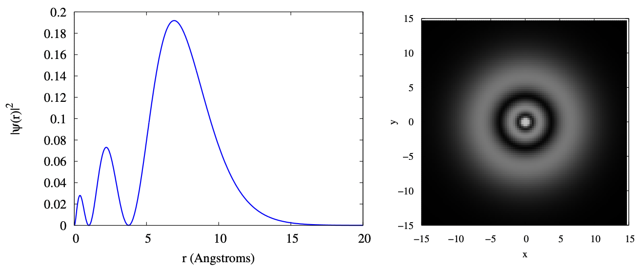
As we move to the 3s orbital, we have to expand the limits of our plots, as the electron is starting to have more and more probability to be at greater radius. In the plots below, you can see that the electron cloud still has reasonable probability density at a radius of 15 Angstroms. You can also see that the 3s orbital is three concentric fuzzy spherical shells; equivalently, the radial function has three bumps. Again, sizes are in Angstroms.