2.10: Harmonic Oscillator- Brute Force Approach

To complete our review of the basic 1D wave mechanics, we have to consider the famous harmonic oscillator, i.e. a 1D particle moving in the quadratic-parabolic potential (111), so that the stationary Schrödinger equation (53) is \[-\frac{\hbar^{2}}{2 m} \frac{d^{2} \psi}{d x^{2}}+\frac{m \omega_{0}^{2} x^{2}}{2} \psi=E \psi\] Conceptually, on the background of the fascinating quantum effects discussed in the previous sections, this is not a very interesting system: Eq. (261) is a standard 1D eigenproblem, resulting in a discrete energy spectrum \(E_{n}\), with smooth eigenfunctions \(\psi_{n}(x)\) vanishing at \(x \rightarrow \pm \infty\) (because the potential energy tends to infinity there) \({ }^{86}\) However, as we will repeatedly see later in the course, this problem’s solutions have an enormous range of applications, so we have to know their basic properties.

The direct analytical solution of the problem is not very simple (see below), so let us start by trying some indirect approaches to it. First, as was discussed in Sec. 4, the WKB-approximation-based Wilson-Sommerfeld quantization rule (110), applied to this potential, yields the eigenenergy spectrum (114). With the common quantum number convention, this result is \[E_{n}=\hbar \omega_{0}\left(n+\frac{1}{2}\right), \quad \text { with } n=0,1,2, \ldots,\] so that (in contrast to the 1D rectangular potential well) the ground-state energy corresponds to \(n=0\). However, as was discussed in the end of Sec. 4, for the quadratic potential (111) the WKB approximation’s conditions are strictly satisfied only at \(E_{n} \gg \hbar \omega_{0}\), so that so far we can only trust Eq. (262) for high levels, with \(n>>1\), rather than for the (most important) ground state.

This is why let me use Eq. (261) to demonstrate another approximate approach, called the variational method, whose simplest form is aimed at finding ground states. The method is based on the following observation. (Here I am presenting its 1D wave mechanics form, though the method is much more general.) Let \(\psi_{n}\) be the exact, full, and orthonormal set of stationary wavefunctions of the system under study, and \(E_{n}\) the set of the corresponding energy levels, satisfying Eq. (1.60): \[\hat{H} \psi_{n}=E_{n} \psi_{n} .\] Then we may use this set for the unique expansion of an arbitrary trial wavefunction \(\psi_{\text {trial }}\) : \[\psi_{\text {tral }}=\sum_{n} \alpha_{n} \psi_{n}, \quad \text { so that } \psi_{\text {trial }}^{*}=\sum_{n} \alpha_{n}^{*} \psi_{n}^{*},\] where \(\alpha_{n}\) are some (generally, complex) coefficients. Let us require the trial function to be normalized, using the condition (1.66) of orthonormality of the eigenfunctions \(\psi_{n}\) : \[\int \psi_{\text {trial }}^{*} \psi_{\text {trial }} d^{3} x \equiv \sum_{n, n^{\prime}} \int \alpha_{n}^{*} \psi_{n}^{*} \alpha_{n^{\prime}} \psi_{n^{\prime}} d^{3} x \equiv \sum_{n, n^{\prime}} \alpha_{n^{\prime}} \alpha_{n}^{*} \int \psi_{n}^{*} \psi_{n^{\prime}} d^{3} x \equiv \sum_{n, n^{\prime}} \alpha_{n^{\prime}} \alpha_{n}^{*} \delta_{n, n^{\prime}} \equiv \sum_{n} W_{n}=1,\] where each of the coefficients \(W_{n}\), defined as \[W_{n} \equiv \alpha_{n}^{*} \alpha_{n} \equiv\left|\alpha_{n}\right|^{2} \geq 0,\] may be interpreted as the probability for the particle, in the \(n^{\text {th }}\) trial state, to be found in the \(n^{\text {th }}\) genuine stationary state. Now let us use Eq. (1.23) for a similar calculation of the expectation value of the system’s Hamiltonian in the trial state: \({ }^{87}\) \[\begin{aligned} \langle H\rangle_{\text {trial }} &=\int \psi_{\text {trial }}^{*} \hat{H} \psi_{\text {trial }} d^{3} x \equiv \sum_{n, n^{\prime}} \int \alpha_{n}^{*} \psi_{n}^{*} \hat{H} \alpha_{n^{\prime}} \psi_{n^{\prime}} d^{3} x \equiv \sum_{n, n^{\prime}} \alpha_{n^{\prime}} \alpha_{n}^{*} E_{n^{\prime}} \int \psi_{n}^{*} \psi_{n^{\prime}} d^{3} x \\ & \equiv \sum_{n, n^{\prime}} \alpha_{n^{\prime}} \alpha_{n}^{*} E_{n^{\prime}} \delta_{n, n^{\prime}} \equiv \sum_{n} W_{n} E_{n} . \end{aligned}\] Since the exact ground state energy \(E_{\mathrm{g}}\) is, by definition, the lowest one of the set \(E_{n}\), i.e. \(E_{n} \geq E_{\mathrm{g}}\), Eqs. (265) and (267) yield the following inequality: \[\langle H\rangle_{\text {trial }} \geq \sum_{n} W_{n} E_{\mathrm{g}} \equiv E_{\mathrm{g}} \sum_{n} W_{n}=E_{\mathrm{g}}\] Thus, the genuine ground state energy of the system is always lower than (or equal to) its energy in any trial state. Hence, if we make several attempts with reasonably selected trial wavefunctions, we may expect the lowest of the results to approximate the genuine ground state energy reasonably well. Even more conveniently, if we select some reasonable class of trial wavefunctions dependent on a free parameter \(\lambda\), then we may use the necessary condition of the minimum of \(\langle H\rangle_{\text {trial }}\), \[\frac{\partial\langle H\rangle_{\text {trial }}}{\partial \lambda}=0,\] to find the closest of them to the genuine ground state. Even better results may be obtained using trial wavefunctions dependent on several parameters. Note, however, that the variational method does not tell us how exactly the trial function should be selected, or how close its final result is to the genuine ground-state function. In this sense, this method has "uncontrollable accuracy", and differs from both the WKB approximation and the perturbation methods (to be discussed in Chapter 6), for which we have certain accuracy criteria. Because of this drawback, the variational method is typically used as the last resort - though sometimes (as in the example that follows) it works remarkably well. 88

Let us apply this method to the harmonic oscillator. Since the potential (111) is symmetric with respect to point \(x=0\), and continuous at all points (so that, according to Eq. (261), \(d^{2} \psi / d x^{2}\) has to be continuous as well), the most natural selection of the ground-state trial function is the Gaussian function \[\psi_{\text {trial }}(x)=C \exp \left\{-\lambda x^{2}\right\},\] with some real \(\lambda>0\). The normalization coefficient \(C\) may be immediately found either from the standard Gaussian integration of \(\left|\psi_{\text {trial }}\right|^{2}\), or just from the comparison of this expression with Eq. (16), in which \(\lambda=1 /(2 \delta x)^{2}\), i.e. \(\delta x=1 / 2 \lambda^{1 / 2}\), giving \(|C|^{2}=(2 \lambda / \pi)^{1 / 2}\). Now the expectation value of the particle’s Hamiltonian, \[\hat{H}=\frac{\hat{p}^{2}}{2 m}+U(x)=-\frac{\hbar^{2}}{2 m} \frac{d^{2}}{d x^{2}}+\frac{m \omega_{0}^{2} x^{2}}{2}\] in the trial state, may be calculated as \[\begin{aligned} \langle H\rangle_{\text {trial }} & \equiv \int_{-\infty}^{+\infty} \psi_{\text {trial }}^{*}\left(-\frac{\hbar^{2}}{2 m} \frac{d^{2}}{d x^{2}}+\frac{m \omega_{0}^{2} x^{2}}{2}\right) \psi_{\text {trial }} d x \\ &=\left(\frac{2 \lambda}{\pi}\right)^{1 / 2}\left[\frac{\hbar^{2} \lambda}{m} \int_{0}^{\infty} \exp \left\{-2 \lambda x^{2}\right\} d x+\left(\frac{m \omega_{0}^{2}}{2}-\frac{2 \hbar^{2} \lambda^{2}}{m}\right) \int_{0}^{\infty} x^{2} \exp \left\{-2 \lambda x^{2}\right\} d x\right] \end{aligned}\] Both involved integrals are of the same well-known Gaussian type,\({ }^{89}\) giving \[\langle H\rangle_{\text {trial }}=\frac{\hbar^{2}}{2 m} \lambda+\frac{m \omega_{0}^{2}}{8 \lambda} .\] As a function of \(\lambda\), this expression has a single minimum at the value \(\lambda_{\text {opt }}\) that may be found from the requirement (269), giving \(\lambda_{\text {opt }}=m \omega_{0} / 2 \hbar\). The resulting minimum of \(\langle H\rangle_{\text {trial }}\) is exactly equal to groundstate energy following from Eq. (262),

Such a coincidence of results of the WKB approximation and the variational method is rather unusual, and implies (though does not strictly prove) that Eq. (274) is exact. As a minimum, this coincidence gives a strong motivation to plug the trial wavefunction \((270)\), with \(\lambda=\lambda_{\text {opt }}\), i.e. \[\psi_{0}=\left(\frac{m \omega_{0}}{\pi \hbar}\right)^{1 / 4} \exp \left\{-\frac{m \omega_{0} x^{2}}{2 \hbar}\right\},\] and the energy (274), into the Schrödinger equation (261). Such substitution \({ }^{90}\) shows that the equation is indeed exactly satisfied.

According to Eq. (275), the characteristic scale of the wavefunction’s spatial spread \({ }^{91}\) is \[x_{0} \equiv\left(\frac{\hbar}{m \omega_{0}}\right)^{1 / 2}\] Due to the importance of this scale, let us give its crude estimates for several representative systems: \({ }^{92}\)

(i) For atom-bound electrons in solids and fluids, \(m \sim 10^{-30} \mathrm{~kg}\), and \(\omega_{0} \sim 10^{15} \mathrm{~s}^{-1}\), giving \(x_{0} \sim 0.3\) \(\mathrm{nm}\), of the order of the typical inter-atomic distances in condensed matter. As a result, classical mechanics is not valid at all for the analysis of their motion.

(ii) For atoms in solids, \(m \approx 10^{-24}-10^{-26} \mathrm{~kg}\), and \(\omega_{0} \sim 10^{13} \mathrm{~s}^{-1}\), giving \(x_{0} \sim 0.01-0.1 \mathrm{~nm}\), i.e. somewhat smaller than inter-atomic distances. Because of that, the methods based on classical mechanics (e.g., molecular dynamics) are approximately valid for the analysis of atomic motion, though they may miss some fine effects exhibited by lighter atoms - e.g., the so-called quantum diffusion of hydrogen atoms, due to their tunneling through the energy barriers of the potential profile created by other atoms.

(iii) Recently, the progress of patterning technologies has enabled the fabrication of high-quality micromechanical oscillators consisting of zillions of atoms. For example, the oscillator used in one of the pioneering experiments in this field \({ }^{93}\) was a \(\sim 1-\mu \mathrm{m}\) thick membrane with a \(60-\mu \mathrm{m}\) diameter, and had \(m \sim 2 \times 10^{-14} \mathrm{~kg}\) and \(\omega_{0} \sim 3 \times 10^{10} \mathrm{~s}^{-1}\), so that \(x_{0} \sim 4 \times 10^{-16} \mathrm{~m}\). It is remarkable that despite such extreme smallness of \(x_{0}\) (much smaller than not only any atom but even any atomic nucleus!), quantum states of such oscillators may be manipulated and measured, using their coupling to electromagnetic (in particular, optical) resonant cavities. \({ }^{94}\)Returning to the Schrödinger equation (261), in order to analyze its higher eigenstates, we will need more help from mathematics. Let us recast this equation into a dimensionless form by introducing the dimensionless variable \(\xi \equiv x / x_{0}\). This gives \[-\frac{d^{2} \psi}{d \xi^{2}}+\xi^{2} \psi=\varepsilon \psi\] where \(\varepsilon \equiv 2 E / \hbar \omega_{0}=E / E_{0}\). In this notation, the ground-state wavefunction (275) is proportional to \(\exp \{-\) \(\left.\xi^{2} / 2\right\}\). Using this clue, let us look for solutions to Eq. (277) in the form \[\psi=C \exp \left\{-\frac{\xi^{2}}{2}\right\} H(\xi),\] where \(H(\xi)\) is a new function, and \(C\) is the normalization constant. With this substitution, Eq. (277) yields \[\frac{d^{2} H}{d \xi^{2}}-2 \xi \frac{d H}{d \xi}+(\varepsilon-1) H=0\] It is evident that \(H=\) const and \(\varepsilon=1\) is one of its solutions, describing the ground-state eigenfunction (275) and energy (274), but what are the other eigenstates and eigenvalues? Fortunately, the linear differential equation (274) was studied in detail in the mid-1800s by C. Hermite who has shown that all its eigenvalues are given by the set \[\varepsilon_{n}-1=2 n, \quad \text { with } n=0,1,2, \ldots,\] so that Eq. (262) is indeed exact for any \(n .95\) The eigenfunction of Eq. (279), corresponding to the eigenvalue \(\varepsilon_{n}\), is a polynomial (called the Hermite polynomial) of degree \(n\), which may be most conveniently calculated using the following explicit formula: \[\ \text{Hermite polynomials}\quad\quad\quad\quad H_{n}=(-1)^{n} \exp \left\{\xi^{2}\right\} \frac{d^{n}}{d \xi^{n}} \exp \left\{-\xi^{2}\right\}.\] It is easy to use this formula to spell out several lowest-degree polynomials - see Fig. 35a: \[H_{0}=1, \quad H_{1}=2 \xi, \quad H_{2}=4 \xi^{2}-2, \quad H_{3}=8 \xi^{3}-12 \xi, \quad H_{4}=16 \xi^{4}-48 \xi^{2}+12, \ldots\]

Fig. 2.35. (a) A few lowest Hermite polynomials and (b) the corresponding eigenenergies (horizontal dashed lines) and eigenfunctions (solid lines) of the harmonic oscillator. The black dashed curve shows the potential profile \(U(x)\) drawn on the same scale as the energies \(E_{n}\), so that its crossings with the energy levels correspond to classical turning points.

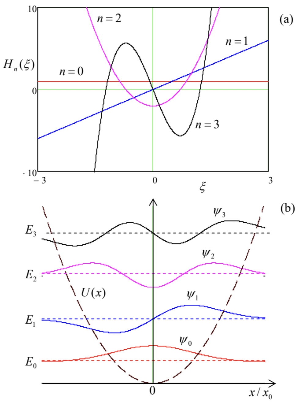
The properties of these polynomials, which most important for applications, are as follows:

(i) the function \(H_{n}(\xi)\) has exactly \(n\) zeros (its plot crosses the \(\xi\)-axis exactly \(n\) times); as a result, the "parity" (symmetry-antisymmetry) of these functions alternates with \(n\), and

(ii) the polynomials are mutually orthonormal in the following sense: \[\int_{-\infty}^{+\infty} H_{n}(\xi) H_{n^{\prime}}(\xi) \exp \left\{-\xi^{2}\right\} d \xi=\pi^{1 / 2} 2^{n} n ! \delta_{n, n^{\prime}} .\] Using the last property, we may readily calculate, from Eq. (278), the normalized eigenfunctions \(\psi_{n}(x)\) of the harmonic oscillator - see Fig.35b: \[\psi_{n}(x)=\frac{1}{\left(2^{n} n !\right)^{1 / 2} \pi^{1 / 4} x_{0}^{1 / 2}} \exp \left\{-\frac{x^{2}}{2 x_{0}^{2}}\right\} H_{n}\left(\frac{x}{x_{0}}\right) .\] At this point, it is instructive to compare these eigenfunctions with those of a \(1 \mathrm{D}\) rectangular potential well, with its ultimately hard walls - see Fig. 1.8. Let us list their common features:

(i) The wavefunctions oscillate in the classically allowed regions with \(E_{n}>U(x)\), while dropping exponentially beyond the boundaries of that region. (For the rectangular well with infinite walls, the latter regions are infinitesimally narrow.)

(ii) Each step up the energy level ladder increases the number of the oscillation halfwaves (and hence the number of its zeros), by one. \({ }^{96}\)

And here are the major features specific for soft (e.g., the quadratic-parabolic) confinement:

(i) The spatial spread of the wavefunction grows with \(n\), following the gradual widening of the classically allowed region.

(ii) Correspondingly, \(E_{n}\) exhibits a slower growth than the \(E_{n} \propto n^{2}\) law given by Eq. (1.85), because the gradual reduction of spatial confinement moderates the kinetic energy’s growth.

Unfortunately, the "brute-force" approach to the harmonic oscillator problem, discussed above, is not too appealing. First, the proof of Eq. (281) is rather longish - so I do not have time/space for it. More importantly, it is hard to use Eq. (284) for the calculation of the expectation values of observables including the so-called matrix elements of the system - as we will see in Chapter 4, virtually the only numbers important for most applications. Finally, it is also almost evident that there has to be some straightforward math leading to any formula as simple as Eq. (262) for \(E_{n}\). Indeed, there is a much more efficient, operator-based approach to this problem; it will be described in Sec. \(5.4\).

---

\({ }^{85}\) See, e.g., CM Sec. 5.4.

\({ }^{86}\) The stationary state of the harmonic oscillator (which, as will be discussed in Secs. \(5.4\) and \(7.1\), may be considered as the state with a definite number of identical bosonic excitations) are sometimes called Fock states after Vladimir Aleksandrovich Fock. (This term is also used in a more general sense, for definite-particle-number states of systems with indistinguishable bosons of any kind - see Sec. 8.3.)

\({ }^{87}\) It is easy (and hence left for the reader) to show that the uncertainty \(\delta H\) in any state of a Hamiltonian system, including the trial state (264), vanishes, so that the \(\langle H\rangle_{\text {trial }}\) may be interpreted as the definite energy of the state. For our current goals, however, this fact is not important.

\({ }^{88}\) The variational method may be used also to estimate the first excited state (or even a few lowest excited states) of the system, by requiring the new trial function to be orthogonal to the previously calculated eigenfunctions of the lower-energy states. However, the method’s error typically grows with the state number.

\({ }^{89}\) See, e.g., MA Eqs. (6.9b) and (6.9c).

\({ }^{90}\) Actually, this is a twist of one of the tasks of Problem \(1.12 .\)

\({ }^{91}\) Quantitatively, as was already mentioned in \(\operatorname{Sec} .2 .1, x_{0}=\sqrt{2} \delta x=\left\langle 2 x^{2}\right\rangle^{1 / 2} .\)

\({ }^{92}\) By order of magnitude, such estimates are valid even for the systems whose dynamics is substantially different from that of harmonic oscillators, if a typical frequency of quantum transitions is taken for \(\omega_{0}\).

\({ }^{93} \mathrm{~A}\). O’Connell et al., Nature 464, 697 (2010).

\({ }^{94}\) See a review of such experiments by M. Aspelmeyer et al., Rev. Mod. Phys. 86, 1391 (2014), and also recent experiments with nanoparticles placed in much "softer" potential wells - e.g., by U. Delić et al., Science 367, 892 (2020).

\({ }^{95}\) Perhaps the most important property of this energy spectrum is that it is equidistant: \(E_{n+1}-E_{n}=\hbar \omega_{0}=\) const.

\({ }^{96}\) In mathematics, a slightly more general statement, valid for a broader class of ordinary linear differential equations, is frequently called the Sturm oscillation theorem, and is a part of the Sturm-Liouville theory of such equations - see, e.g., Chapter 10 in the handbook by G. Arfken et al., cited in MA Sec. \(16 .\)