4.8: Exercise Problems

4.1. Prove that if \(\hat{A}\) and \(\hat{B}\) are linear operators, and \(C\) is a \(c\)-number, then:

(i) \(\left(\hat{A}^{\dagger}\right)^{\dagger}=\hat{A}\);

(ii) \((C \hat{A})^{\dagger}=C^{*} \hat{A}^{\dagger} ;\)

(iii) \((\hat{A} \hat{B})^{\dagger}=\hat{B}^{\dagger} \hat{A}^{\dagger} ;\)

(iv) the operators \(\hat{A} \hat{A}^{\dagger}\) and \(\hat{A}^{\dagger} \hat{A}\) are Hermitian.

4.2. Prove that for any linear operators \(\hat{A}, \hat{B}, \hat{C}\), and \(\hat{D}\), \[[\hat{A} \hat{B}, \hat{C} \hat{D}]=\hat{A}\{\hat{B}, \hat{C}\} \hat{D}-\hat{A} \hat{C}\{\hat{B}, \hat{D}\}+\{\hat{A}, \hat{C}\} \hat{D} \hat{B}-\hat{C}\{\hat{A}, \hat{D}\} \hat{B}\]

4.3. Calculate all possible binary products \(\sigma_{j} \sigma_{j^{\prime}}\) (for \(j, j^{\prime}=x, y, z\) ) of the Pauli matrices, defined by Eqs. (105), and their commutators and anticommutators (defined similarly to those of the corresponding operators). Summarize the results, using the Kronecker delta and Levi-Civita permutation symbols. \({ }^{54}\)

4.4. Calculate the following expressions,

(i) \((\mathbf{c} \cdot \boldsymbol{\sigma})^{n}\), and then

(ii) \((b \mathrm{I}+\mathbf{c} \cdot \mathbf{\sigma})^{n}\),

for the scalar product \(\mathbf{c} \cdot \boldsymbol{\sigma}\) of the Pauli matrix vector \(\boldsymbol{\sigma} \equiv \mathbf{n}_{x} \sigma_{x}+\mathbf{n}_{y} \sigma_{y}+\mathbf{n}_{z} \sigma_{z}\) by an arbitrary \(c\)-number geometric vector \(\mathbf{c}\), where \(n \geq 0\) is an integer, and \(b\) is an arbitrary scalar \(c\)-number.

Hint: For task (ii), you may like to use the binomial theorem, \({ }^{55}\) and then transform the result in a way enabling you to use the same theorem backward.

4.5. Use the solution of the previous problem to derive Eqs. (2.191) for the transparency \(\mathscr{T}\) of a system of \(N\) similar, equidistant, delta-functional potential barriers.

4.6. Use the solution of Problem 4(i) to spell out the following matrix: \(\exp \{i \theta \mathbf{n} \cdot \boldsymbol{\sigma}\}\), where \(\sigma\) is the 3D vector (117) of the Pauli matrices, \(\mathbf{n}\) is a \(c\)-number geometric vector of unit length, and \(\theta\) is a \(c-\) number scalar.

4.7. Use the solution of Problem 4(ii) to calculate \(\exp \{\mathrm{A}\}\), where \(\mathrm{A}\) is an arbitrary \(2 \times 2\) matrix.

4.8. Express all elements of the matrix \(\mathrm{B} \equiv \exp \{\mathrm{A}\}\) explicitly via those of the \(2 \times 2\) matrix \(\mathrm{A}\). Spell out your result for the following matrices: \[\mathrm{A}=\left(\begin{array}{ll} a & a \\ a & a \end{array}\right), \quad \mathrm{A}^{\prime}=\left(\begin{array}{ll} i \varphi & i \varphi \\ i \varphi & i \varphi \end{array}\right),\] with real \(a\) and \(\varphi\).

4.9. Prove that for arbitrary square matrices \(\mathrm{A}\) and \(\mathrm{B}\), \[\operatorname{Tr}(\mathrm{AB})=\operatorname{Tr}(\mathrm{BA}) \text {. }\] Is each diagonal element \((A B)_{j j}\) necessarily equal to \((B A)_{j j}\) ?

4.10. Calculate the trace of the following \(2 \times 2\) matrix: \[\mathrm{A} \equiv(\mathbf{a} \cdot \boldsymbol{\sigma})(\mathbf{b} \cdot \boldsymbol{\sigma})(\mathbf{c} \cdot \boldsymbol{\sigma}),\] where \(\sigma\) is the Pauli matrix vector, while \(\mathbf{a}, \mathbf{b}\), and \(\mathbf{c}\) are arbitrary \(c\)-number vectors.

4.11. Prove that the matrix trace of an arbitrary operator does not change at its arbitrary unitary transformation.

4.12. Prove that for any two full and orthonormal bases \(\{u\}\) and \(\{v\}\) of the same Hilbert space, \[\operatorname{Tr}\left(\left|u_{j}\right\rangle\left\langle v_{j^{\prime}}\right|\right)=\left\langle v_{j^{\prime}} \mid u_{j}\right\rangle .\] 4.13. Is the \(1 \mathrm{D}\) scattering matrix \(\mathrm{S}\), defined by Eq. (2.124), unitary? What about the 1D transfer matrix T defined by Eq. (2.125)?

4.14. Calculate the trace of the following matrix: \[\exp \{i \mathbf{a} \cdot \boldsymbol{\sigma}\} \exp \{i \mathbf{b} \cdot \boldsymbol{\sigma}\},\] where \(\sigma\) is the Pauli matrix vector, while \(\mathbf{a}\) and \(\mathbf{b}\) are \(c\)-number geometric vectors.

4.15. Prove the following vector-operator identity: \[(\boldsymbol{\sigma} \cdot \hat{\mathbf{r}})(\boldsymbol{\sigma} \cdot \hat{\mathbf{p}})=\mathrm{I} \hat{\mathbf{r}} \cdot \hat{\mathbf{p}}+i \boldsymbol{\sigma} \cdot(\hat{\mathbf{r}} \times \hat{\mathbf{p}}),\] where \(\sigma\) is the Pauli matrix vector, and \(\mathrm{I}\) is the \(2 \times 2\) identity matrix. Hint: Take into account that the vector operators \(\hat{\mathbf{r}}\) and \(\hat{\mathbf{p}}\) are defined in the orbital-motion Hilbert space, different from that of the Pauli vector-matrix \(\sigma\), and hence commute with it - even though they do not commute with each other.

4.16. Let \(A_{j}\) be eigenvalues of some operator \(\hat{A}\). Express the following two sums, \[\Sigma_{1} \equiv \sum_{j} A_{j}, \quad \Sigma_{2} \equiv \sum_{j} A_{j}^{2},\] via the matrix elements \(A_{j j}\) ’ of this operator in an arbitrary basis.

4.17. Calculate \(\left\langle\sigma_{z}\right\rangle\) of a spin-1/2 in the quantum state with the following ket-vector: \[|\alpha\rangle=\text { const } \times(|\uparrow\rangle+|\downarrow\rangle+|\rightarrow\rangle+|\leftarrow\rangle) \text {, }\] where \((\uparrow, \downarrow)\) and \((\rightarrow, \leftarrow)\) are the eigenstates of the Pauli matrices \(\sigma_{z}\) and \(\sigma_{x}\), respectively.

Hint: Double-check whether your solution is general.

4.18. A spin- \(1 / 2\) is fully polarized in the positive \(z\)-direction. Calculate the probabilities of the alternative outcomes of a perfect Stern-Gerlach experiment with the magnetic field oriented in an arbitrary different direction, performed on a particle in this spin state.

4.19. In a certain basis, the Hamiltonian of a two-level system is described by the matrix \[\mathrm{H}=\left(\begin{array}{cc} E_{1} & 0 \\ 0 & E_{2} \end{array}\right), \quad \text { with } E_{1} \neq E_{2},\] while the operator of some observable \(A\) of this system, by the matrix \[\mathrm{A}=\left(\begin{array}{ll} 1 & 1 \\ 1 & 1 \end{array}\right) \text {. }\] For the system’s state with the energy definitely equal to \(E_{1}\), find the possible results of measurements of the observable \(A\) and the probabilities of the corresponding measurement outcomes.

4.20. Certain states \(u_{1,2,3}\) form an orthonormal basis of a system with the following Hamiltonian \[\hat{H}=-\delta\left(\left|u_{1}\right\rangle\left\langle u_{2}|+| u_{2}\right\rangle\left\langle u_{3}|+| u_{3}\right\rangle\left\langle u_{1}\right|\right)+\text { h.c., }\] where \(\delta\) is a real constant, and h.c. means the Hermitian conjugate of the previous expression. Calculate its stationary states and energy levels. Can you relate this system to any other(s) discussed earlier in the course?

4.21. Guided by Eq. (2.203), and by the solutions of Problems \(3.11\) and \(4.20\), suggest a Hamiltonian describing particle’s dynamics in an infinite \(1 \mathrm{D}\) chain of similar potential wells in the tightbinding approximation, in the bra-ket formalism. Verify that its eigenstates and eigenvalues correspond to those discussed in Sec. \(2.7\). 4.22. Calculate eigenvectors and eigenvalues of the following matrices: \[\mathrm{A}=\left(\begin{array}{lll} 0 & 1 & 0 \\ 1 & 0 & 1 \\ 0 & 1 & 0 \end{array}\right), \quad \mathrm{B}=\left(\begin{array}{llll} 0 & 0 & 0 & 1 \\ 0 & 0 & 1 & 0 \\ 0 & 1 & 0 & 0 \\ 1 & 0 & 0 & 0 \end{array}\right)\] \(\underline{4.23}\). A certain state \(\gamma\) is an eigenstate of each of two operators, \(\hat{A}\) and \(\hat{B}\). What can be said about the corresponding eigenvalues \(a\) and \(b\), if the operators anticommute?

4.24. Derive the differential equation for the time evolution of the expectation value of an observable, using both the Schrödinger picture and the Heisenberg picture of quantum dynamics.

4.25. At \(t=0\), a spin- \(1 / 2\) whose interaction with an external field is described by the Hamiltonian \[\hat{H}=\mathbf{c} \cdot \hat{\boldsymbol{\sigma}} \equiv c_{x} \hat{\sigma}_{x}+c_{y} \hat{\sigma}_{y}+c_{z} \hat{\sigma}_{z}\] (where \(c_{x, y, z}\) are real \(c\)-number constants, and \(\hat{\sigma}_{x, y, z}\) are the Pauli operators), was in the state \(\uparrow\), one of the two eigenstates of \(\hat{\sigma}_{z}\). In the Schrödinger picture, calculate the time evolution of:

(i) the ket-vector \(|\alpha\rangle\) of the spin (in any time-independent basis you like),

(ii) the probabilities to find the spin in the states \(\uparrow\) and \(\downarrow\), and

(iii) the expectation values of all three Cartesian components \(\left(\hat{S}_{x}\right.\), etc. \()\) of the spin vector.

Analyze and interpret the results for the particular case \(c_{y}=c_{z}=0\).

Hint: Think about the best basis to use for the solution.

4.26. For the same system as in the previous problem, use the Heisenberg picture to calculate the time evolution of:

(i) all three Cartesian components of the spin operator \(\hat{\mathbf{S}}_{\mathrm{H}}(t)\), and

(ii) the expectation values of the spin components.

Compare the latter results with those of the previous problem.

4.27. For the same system as in the two last problems, calculate matrix elements of the operator \(\hat{\sigma}_{z}\) in the basis of the stationary states of the system.

4.28. In the Schrödinger picture of quantum dynamics, certain three operators satisfy the following commutation relation: \[[\hat{A}, \hat{B}]=\hat{C} \text {. }\] What is their relation in the Heisenberg picture, at a certain time instant \(t\) ?

4.29. Prove the Bloch theorem given by either Eq. (3.107) or Eq. (3.108). Hint: Consider the translation operator \(\hat{\tau}_{\mathrm{R}}\) defined by the following result of its action on an arbitrary function \(f(\mathbf{r})\) : \[\hat{\tau}_{\mathrm{R}} f(\mathbf{r})=f(\mathbf{r}+\mathbf{R}),\] for the case when \(\mathbf{R}\) is an arbitrary vector of the Bravais lattice (3.106). In particular, analyze the commutation properties of this operator, and apply them to an eigenfunction \(\psi(\mathbf{r})\) of the stationary Schrödinger equation for a particle moving in the 3D periodic potential described by Eq. (3.105).

4.30. A constant force \(F\) is applied to an (otherwise free) 1D particle of mass \(m\). Calculate the stationary wavefunctions of the particle in:

(i) the coordinate representation, and

(ii) the momentum representation.

Discuss the relation between the results.

4.31. Use the momentum representation to re-solve the problem discussed at the beginning of Sec. 2.6, i.e. calculate the eigenenergy of a 1D particle of mass \(m\), localized in a very short potential well of "weight" \(w\).

4.32. The momentum representation of a certain operator of \(1 \mathrm{D}\) orbital motion is \(p^{-1}\). Find its coordinate representation.

4.33. For a particle moving in a 3D periodic potential, develop the bra-ket formalism for the qrepresentation, in which a complex amplitude similar to \(a_{q}\) in Eq. (2.234) (but generalized to 3D and all energy bands) plays the role of the wavefunction. In particular, calculate the operators \(\mathbf{r}\) and \(\mathbf{v}\) in this representation, and use the result to prove Eq. (2.237) for the 1D case in the low-field limit.

4.34. A uniform, time-independent magnetic field \(\mathscr{R}\) is induced in one semispace, while the other semi-space is field-free, with a sharp, plane boundary between these two regions. A monochromatic beam of non-relativistic, electricallyneutral spin- \(1 / 2\) particles with a gyromagnetic ratio \(\gamma \neq 0,{ }^{56}\) in a certain spin state and with a kinetic energy \(E\), is incident on this boundary, from the field-free side, under angle \(\theta\) - see figure on the right. Calculate the coefficient of particle reflection from the boundary.

---

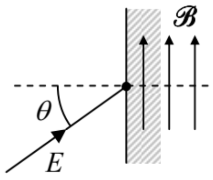
\({ }^{56}\) The fact that \(\gamma\) may be different from zero even for electrically-neutral particles, such as neutrons, is explained by the Standard Model of the elementary particles, in which a neutron "consists" (in a broad sense of the word) of three electrically-charged quarks with zero net charge.