5.5: Glauber States and Squeezed States

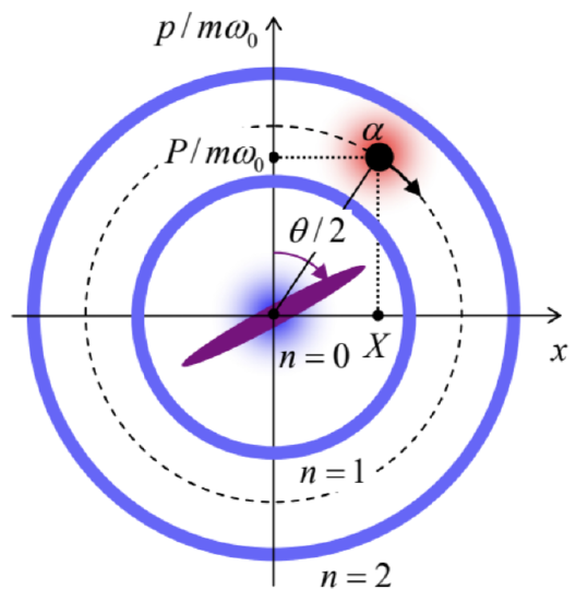
There is a huge difference between a quantum stationary (Fock) state of the oscillator and its classical state. Indeed, let us write the well known classical equations of motion of the oscillator (using capital letters to distinguish classical variables from the arguments of quantum wavefunctions): \({ }^{34}\) \[\dot{X}=\frac{P}{m}, \quad \dot{P}=-\frac{\partial U}{\partial x}=-m \omega_{0}^{2} X .\] On the so-called phase plane, with the Cartesian coordinates \(x\) and \(p\), these equations describe a clockwise rotation of the representation point \(\{X(t), P(t)\}\) along an elliptic trajectory starting from the initial point \(\{X(0), P(0)\}\). (The normalization of the momentum by \(m \omega_{0}\), similar to the one performed by the second of Eqs. (63), makes this trajectory pleasingly circular, with a constant radius equal to the oscillations amplitude \(A\), corresponding to the constant full energy \[E=\frac{m \omega_{0}^{2}}{2} A^{2}, \quad \text { with } A^{2}=[X(t)]^{2}+\left[\frac{P(t)}{m \omega_{0}}\right]^{2}=\text { const }=[X(0)]^{2}+\left[\frac{P(0)}{m \omega_{0}}\right]^{2},\] determined by the initial conditions - see Fig. 8.)

Fig. 5.8. Representations of various states of a harmonic oscillator on the phase plane. The bold black point represents a classical state with the complex amplitude \(\alpha\), with the dashed line showing its trajectory. The (very imperfect) classical images of the Fock states with \(n=0\), 1 , and 2 are shown in blue. The blurred red spot is the (equally schematic) image of the Glauber state \(\alpha\). Finally, the magenta elliptical spot is a classical image of a squeezed ground state - see below. Arrows show the direction of the states’ evolution in time.

For the forthcoming comparison with quantum states, it is convenient to describe this classical motion by the following dimensionless complex variable \[\alpha(t) \equiv \frac{1}{\sqrt{2} x_{0}}\left[X(t)+i \frac{P(t)}{m \omega_{0}}\right] \text {, }\] which is essentially the standard complex-number representation of the representing point’s position on the \(2 \mathrm{D}\) phase plane, with \(|\alpha| \equiv A / \sqrt{2} x_{0}\). With this definition, Eqs. (100) are conveniently merged into one equation, \[\dot{\alpha}=-i \omega_{0} \alpha,\] with an evident, very simple solution \[\alpha(t)=\alpha(0) \exp \left\{-i \omega_{0} t\right\},\] where the constant \(\alpha(0)\) may be complex, and is just the (normalized) classical complex amplitude of oscillations. \({ }^{35}\) This equation describes sinusoidal oscillations of both \(X(t) \propto \operatorname{Re}[\alpha(t)]\) and \(P \propto \operatorname{Im}[\alpha(t)]\), with a phase shift of \(\pi / 2\) between them.

On the other hand, according to the basic Eq. (4.161), the time dependence of a Fock state, as of a stationary state of the oscillator, is limited to the phase factor \(\exp \left\{-i E_{n} t / \hbar\right\}\). This factor drops out at the averaging (4.125) for any observable. As a result, in this state the expectation values of \(x, p\), or of any function thereof are time-independent. (Moreover, as Eqs. (98) show, \(\langle x\rangle=\langle p\rangle=0\).) Taking into account Eqs. (96)-(97), the closest (though very imperfect) geometric image \({ }^{36}\) of such a state on the phase plane is a static circle of the radius \(A_{n}=x_{0}(2 n+1)^{1 / 2}\), along which the wavefunction is uniformly spread \(-\) see the blue rings in Fig. 8. For the ground state \((n=0)\), with the wavefunction \((2.275)\), a better image may be a blurred round spot, of a radius \(\sim x_{0}\), at the origin. (It is easy to criticize such blurring, intended to represent the non-vanishing spreads (99), because it fails to reflect the fact that the total energy of the oscillator in the state, \(E_{0}=\hbar \omega_{0} / 2\) is defined exactly, without any uncertainty.)

So, the difference between a classical state of the oscillator and its Fock state \(n\) is very profound. However, the Fock states are not the only possible quantum states of the oscillator: according to the basic Eq. (4.6), any state described by the ket-vector \[|\alpha\rangle=\sum_{n=0}^{\infty} \alpha_{n}|n\rangle\] with an arbitrary set of (complex) \(c\)-numbers \(\alpha_{n}\), is also its legitimate state, subject only to the normalization condition \(\langle\alpha \mid \alpha\rangle=1\), giving \[\sum_{n=0}^{\infty}\left|\alpha_{n}\right|^{2}=1\] It is natural to ask: could we select the coefficients \(\alpha_{n}\) in such a special way that the state properties would be closer to the classical one; in particular the expectation values \(\langle x\rangle\) and \(\langle p\rangle\) of the coordinate and momentum would evolve in time as the classical values \(X(t)\) and \(P(t)\), while the uncertainties of these observables would be, just as in the ground state, given by Eqs. (99), and hence have the smallest possible uncertainty product, \(\delta x \delta p=\hbar / 2\). Let me show that such a Glauber state, \({ }^{37}\) which is schematically represented in Fig. 8 by a blurred red spot around the classical point \(\{X(t), P(t)\}\), is indeed possible.

Conceptually the simplest way to find the corresponding coefficients \(\alpha_{n}\) would be to calculate \(\langle x\rangle,\langle p\rangle, \delta x\), and \(\delta p\) for an arbitrary set of \(\alpha_{n}\), and then try to optimize these coefficients to reach our goal. However, this problem may be solved much easier using wave mechanics. Indeed, let us consider the following wavefunction: \[\Psi_{\alpha}(x, t)=\left(\frac{m \omega_{0}}{\pi \hbar}\right)^{1 / 2} \exp \left\{-\frac{m \omega_{0}}{2 \hbar}[x-X(t)]^{2}+i \frac{P(t) x}{\hbar}\right\},\] Its comparison with Eqs. (2.275) shows that this is just the ground-state wavefunction, but with the center shifted from the origin into the classical point \(\{X(t), P(t)\}\). A straightforward (though a bit bulky) differentiation over \(x\) and \(t\) shows that it satisfies the oscillator’s Schrödinger equation, provided that the \(c\)-number functions \(X(t)\) and \(P(t)\) obey the classical equations (100). Moreover, a similar calculation shows that the wavefunction (107) also satisfies the Schrödinger equation of an oscillator under the effect of a pulse of a classical force \(F(t)\), provided that the oscillator initially was in its ground state, and that the classical evolution law \(\{X(t), P(t)\}\) in Eq. (107) takes this force into account. \({ }^{38}\) Since for many experimental implementations of the harmonic oscillator, the ground state may be readily formed (for example, by providing a weak coupling of the oscillator to a low-temperature environment), the Glauber state is usually easier to form than any Fock state with \(n>0\). This is why the Glauber states are so important and deserve much discussion.

In such a discussion, there is a substantial place for the bra-ket formalism. For example, to calculate the corresponding coefficients in the expansion (105) by wave-mechanical means, \[\alpha_{n}(t) \equiv\langle n \mid \alpha(t)\rangle=\int d x\langle n \mid x\rangle\langle x \mid \alpha(t)\rangle=\int \psi_{n}^{*}(x) \Psi_{\alpha}(x, t) d x,\] we would need to use not only the simple Eq. (107), but also the Fock state wavefunctions \(\psi_{n}(x)\), which are not very appealing - see Eq. (2.284) again. Instead, this calculation may be readily done in the braket formalism, giving us one important byproduct result as well.

Let us start by expressing the double shift of the ground state (by \(X\) and \(P\) ), which has led us to Eq. (107), in the operator language. Forgetting about the \(P\) for a minute, let us find the translation operator \(\hat{T}_{X}\) that would produce the desired shift of an arbitrary wavefunction \(\psi(x)\) by a \(c\)-number distance \(X\) along the coordinate argument \(x\). This means \[\hat{\tau}_{X} \psi(x) \equiv \psi(x-X) .\] Representing the wavefunction \(\psi\) as the standard wave packet (4.264), we see that \[\hat{\tau}_{X} \psi(x)=\frac{1}{(2 \pi \hbar)^{1 / 2}} \int \varphi(p) \exp \left\{i \frac{p(x-X)}{\hbar}\right\} d p \equiv \frac{1}{(2 \pi \hbar)^{1 / 2}} \int\left[\varphi(p) \exp \left\{-i \frac{p X}{\hbar}\right\}\right] \exp \left\{i \frac{p x}{\hbar}\right\} d p\] Hence, the shift may be achieved by the multiplication of each Fourier component of the packet, with the momentum \(p\), by \(\exp \{-i p X / \hbar\}\). This gives us a hint that the general form of the translation operator, valid in any representation, should be \[\hat{\tau}_{x}=\exp \left\{-i \frac{\hat{p} X}{\hbar}\right\} .\] The proof of this formula is provided merely by the fact that, as we know from Chapter 4 , any operator is uniquely determined by the set of its matrix elements in any full and orthogonal basis, in particular the basis of momentum states \(p\). According to Eq. (110), the analog of Eq. (4.235) for the \(p\)-representation, applied to the translation operator (which is evidently local), is \[\int d p\left\langle p\left|\hat{T}_{X}\right| p^{\prime}\right\rangle \varphi\left(p^{\prime}\right)=\exp \left\{-i \frac{p X}{\hbar}\right\} \varphi(p),\] so that the operator (111) does exactly the job we need it to.

The operator that provides the shift of momentum by a \(c\)-number \(P\) is absolutely similar - with the opposite sign under the exponent, due to the opposite sign of the exponent in the reciprocal Fourier transform, so that the simultaneous shift by both \(X\) and \(P\) may be achieved by the following translation operator: \[\hat{\tau}_{\alpha}=\exp \left\{i \frac{P \hat{x}-\hat{p} X}{\hbar}\right\}\] As we already know, for a harmonic oscillator the creation-annihilation operators are more natural, so that we may use Eqs. (66) to recast Eq. (113) as \[\hat{\tau}_{\alpha}=\exp \left\{\alpha \hat{a}^{\dagger}-\alpha^{*} \hat{a}\right\}, \quad \text { so that } \hat{\tau}_{\alpha}^{\dagger}=\exp \left\{\alpha^{*} \hat{a}-\alpha \hat{a}^{\dagger}\right\}\] where \(\alpha\) (which, generally, may be a function of time) is the \(c\)-number defined by Eq. (102). Now, according to Eq. (107), we may form the Glauber state’s ket-vector just as \[|\alpha\rangle=\hat{T}_{\alpha}|0\rangle .\] This formula, valid in any representation, is very elegant, but using it for practical calculations (say, of the expectation values of observables) is not too easy because of the exponent-of-operators form of the translation operator. Fortunately, it turns out that a much simpler representation for the Glauber state is possible. To show this, let us start with the following general (and very useful) property of exponential functions of an operator argument: if \[[\hat{A}, \hat{B}]=\mu \hat{I},\] (where \(\hat{A}\) and \(\hat{B}\) are arbitrary linear operators, and \(\mu\) is a \(c\)-number), then \(^{39}\) \[\exp \{+\hat{A}\} \hat{B} \exp \{-\hat{A}\}=\hat{B}+\mu \hat{I} .\] Let us apply Eqs. (116)-(117) to two cases, both with \[\hat{A}=\alpha^{*} \hat{a}-\alpha \hat{a}^{\dagger}, \text { so that } \exp \{+\hat{A}\}=\hat{T}_{\alpha}^{\dagger}, \quad \exp \{-\hat{A}\}=\hat{T}_{\alpha}\] First, let us take \(\hat{B}=\hat{I}\); then Eq. (116) is valid with \(\mu=0\), and Eq. (117) yields \[\hat{\tau}_{\alpha}^{\dagger} \hat{T}_{\alpha}=\hat{I},\] This equality means that the translation operator is unitary - not a big surprise, because if we shift a classical point on the phase plane by a complex number \((+\alpha)\) and then by \((-\alpha)\), we certainly must come back to the initial position. Eq. (119) means merely that this fact is true for any quantum state as well.

Second, let us take \(\hat{B}=\hat{a}\); in order to find the corresponding parameter \(\mu\), we must calculate the commutator on the left-hand side of Eq. (116) for this case. Using, at the due stage of the calculation, Eq. (68), we get \[[\hat{A}, \hat{B}]=\left[\alpha^{*} \hat{a}-\alpha \hat{a}^{\dagger}, \hat{a}\right]=-\alpha\left[\hat{a}^{\dagger}, \hat{a}\right]=\alpha \hat{I},\] so that in this case \(\mu=\alpha\), and Eq. (117) yields \[\hat{\tau}_{\alpha}^{\dagger} \hat{a} \hat{T}_{\alpha}=\hat{a}+\alpha \hat{I} .\] We have approached the summit of this beautiful calculation. Let us consider the following operator: \[\hat{\tau}_{\alpha} \hat{\tau}_{\alpha}^{\dagger} \hat{a} \hat{\tau}_{\alpha} .\] Using Eq. (119), we may reduce this product to \(\hat{a} \hat{T}_{\alpha}\), while the application of Eq. (121) to the same expression (122) yields \(\hat{\tau}_{\alpha} \hat{a}+\alpha \hat{T}_{\alpha} .\) Hence, we get the following operator equality: \[\hat{a} \hat{T}_{\alpha}=\hat{T}_{\alpha} \hat{a}+\alpha \hat{T}_{\alpha},\] which may be applied to any state. Now acting by both sides of this equality on the ground state’s ket \(|0\rangle\), and using the fact that \(\hat{a}|0\rangle\) is the null-state, while according to Eq. (115), \(\hat{\tau}_{\alpha}|0\rangle \equiv|\alpha\rangle\), we finally get a very simple and elegant result: \({ }^{40}\) \[\hat{a}|\alpha\rangle=\alpha|\alpha\rangle .\] Thus any Glauber state \(\alpha\) is one of the eigenstates of the annihilation operator, namely the one with the eigenvalue equal to the \(c\)-number parameter \(\alpha\) of the state, i.e. to the complex representation (102) of the classical point which is the center of the Glauber state’s wavefunction. \({ }^{41}\) This fact makes the calculations of all Glauber state properties much simpler. As an example, let us calculate \(\langle x\rangle\) in the Glauber state with some \(c\)-number \(\alpha\) : \[\langle x\rangle=\langle\alpha|\hat{x}| \alpha\rangle=\frac{x_{0}}{\sqrt{2}}\left\langle\alpha\left|\left(\hat{a}+\hat{a}^{\dagger}\right)\right| \alpha\right\rangle \equiv \frac{x_{0}}{\sqrt{2}}\left(\langle\alpha|\hat{a}| \alpha\rangle+\left\langle\alpha\left|\hat{a}^{\dagger}\right| \alpha\right\rangle\right) .\] In the first term in the parentheses, we can apply Eq. (124) directly, while in the second term, we can use the bra-counterpart of that relation, \(\langle\alpha| \hat{a}^{\dagger}=\langle\alpha| \alpha^{*}\). Now assuming that the Glauber state is normalized, \(\langle\alpha \mid \alpha\rangle=1\), and using Eq. (102), we get \[\langle x\rangle=\frac{x_{0}}{\sqrt{2}}\left(\langle\alpha|\alpha| \alpha\rangle+\left\langle\alpha\left|\ldots \alpha^{*}\right| \alpha\right\rangle\right)=\frac{x_{0}}{\sqrt{2}}\left(\alpha+\alpha^{*}\right)=X,\] Acting absolutely similarly, we may verify that \(\langle p\rangle=P\), and that \(\delta x\) and \(\delta p\) do indeed obey Eqs. (99).

As the last sanity check, let us use Eq. (124) to re-calculate the Glauber state’s wavefunction (107). Inner-multiplying both sides of that relation by the bra-vector \(\langle x|\), and using the definition (65a) of the annihilation operator, we get \[\frac{1}{\sqrt{2} x_{0}}\left\langle x \|\left(\hat{x}+i \frac{\hat{p}}{m \omega_{0}}\right) \mid \alpha\right\rangle=\alpha\langle x \mid \alpha\rangle .\] Since \(\langle x|\) is the bra-vector of the eigenstate of the Hermitian operator \(\hat{x}\), they may be swapped, with the operator giving its eigenvalue \(x\); acting on that bra-vector by the (local!) operator of momentum, we have to use it in the coordinate representation - see Eq. (4.245). As a result, we get \[\frac{1}{\sqrt{2} x_{0}}\left(x\langle x \mid \alpha\rangle+\frac{\hbar}{m \omega_{0}} \frac{\partial}{\partial x}\langle x \mid \alpha\rangle\right)=\alpha\langle x \mid \alpha\rangle \text {. }\] But \(\langle x \mid \alpha\rangle\) is nothing else than the Glauber state’s wavefunction \(\Psi_{\alpha}\) so that Eq. (128) gives for it a firstorder differential equation \[\frac{1}{\sqrt{2} x_{0}}\left(x \Psi_{\alpha}+\frac{\hbar}{m \omega_{0}} \frac{\partial}{\partial x} \Psi_{\alpha}\right)=\alpha \Psi_{\alpha} .\] Chasing \(\Psi_{\alpha}\) and \(x\) to the opposite sides of the equation, and using the definition (102) of the parameter \(\alpha\), we can bring this equation to the form (valid at fixed \(t\), and hence fixed \(X\) and \(P\) ): \[\frac{d \Psi_{\alpha}}{\Psi_{\alpha}}=\frac{m \omega_{0}}{\hbar}\left[-x+\left(X+i \frac{P}{m \omega_{0}}\right)\right] d x\] Integrating both parts, we return to Eq. (107).

Now we can use Eq. (124) for finding the coefficients \(\alpha_{n}\) in the expansion (105) of the Glauber state \(\alpha\) in the series over the Fock states \(n\). Plugging Eq. (105) into both sides of Eq. (124), using the second of Eqs. (89) on the left-hand side, and requiring the coefficients at each ket-vector \(|n\rangle\) in both parts of the resulting relation to be equal, we get the following recurrence relation: \[\alpha_{n+1}=\frac{\alpha}{(n+1)^{1 / 2}} \alpha_{n} .\] Applying this relation sequentially for \(n=0,1,2\), etc., we get \[\alpha_{n}=\frac{\alpha^{n}}{(n !)^{1 / 2}} \alpha_{0} .\] Now we can find \(\alpha_{0}\) from the normalization requirement (106), getting \[\left|\alpha_{0}\right|^{2} \sum_{n=0}^{\infty} \frac{|\alpha|^{2 n}}{n !}=1 .\] In this sum, we may readily recognize the Taylor expansion of the function \(\exp \left\{|\alpha|^{2}\right\}\), so that the final result (besides an arbitrary common phase multiplier) is \[|\alpha\rangle=\exp \left\{-\frac{|\alpha|^{2}}{2}\right\} \sum_{n=0}^{\infty} \frac{\alpha^{n}}{(n !)^{1 / 2}}|n\rangle .\] Hence, if the oscillator is in the Glauber state \(\alpha\), the probabilities \(W_{n} \equiv \alpha_{n} \alpha_{n}{ }^{*}\) of finding the system on the \(n^{\text {th }}\) energy level (86) obey the well-known Poisson distribution (Fig. 9): \[W_{n}=\frac{\langle n\rangle^{n}}{n !} e^{-\langle n\rangle},\] where \(\langle n\rangle\) is the statistical average of \(n-\) see Eq. (1.37): \[\langle n\rangle=\sum_{n=0}^{\infty} n W_{n} .\] The result of such summation is not necessarily integer! In our particular case, Eqs. (134)-(136) yield \[\langle n\rangle=|\alpha|^{2} .\]

Fig. 5.9. The Poisson distribution (135) for several values of \(\langle n\rangle\). Note that \(W_{n}\) are defined only for integer values of \(n\); the lines are only guides for the eye.

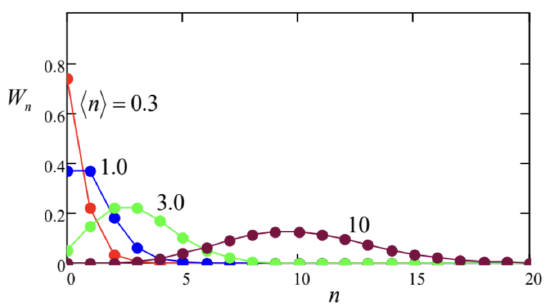
For applications, perhaps the most important mathematical property of this distribution is \[\left\langle\widetilde{n}^{2}\right\rangle \equiv\left\langle(n-\langle n\rangle)^{2}\right\rangle=\langle n\rangle, \quad \text { so that } \delta n \equiv\left\langle\widetilde{n}^{2}\right\rangle^{1 / 2}=\langle n\rangle^{1 / 2}\] Another important property is that at \(\langle n\rangle\rangle>1\), the Poisson distribution approaches the Gaussian ("normal") one, with a small relative r.m.s. uncertainty: \(\delta n /\langle n\rangle<<1-\) the trend clearly visible in Fig. 9 . Now let us discuss the Glauber state’s evolution in time. In the wave-mechanics language, it is completely described by the dynamics (100) of the \(c\)-number shifts \(X(t)\) and \(P(t)\) participating in the wavefunction (107). Note again that, in contrast to the spread of the wave packet of a free particle, discussed in Sec. 2.2, in the harmonic oscillator the Gaussian packet of the special width (99) does not spread at all!

An alternative and equivalent way of dynamics description is to use the Heisenberg equation of motion. As Eqs. (29) and (35) tell us, such equations for the Heisenberg operators of coordinate and momentum have to be similar to the classical equations (100): \[\dot{\hat{x}}_{\mathrm{H}}=\frac{\hat{p}_{\mathrm{H}}}{m}, \quad \dot{\hat{p}}_{\mathrm{H}}=-m \omega_{0}^{2} \hat{x}_{\mathrm{H}} .\] Now using Eqs. (66), for the Heisenberg-picture creation and annihilation operators we get the equations \[\dot{\hat{a}}_{\mathrm{H}}=-i \omega_{0} \hat{a}_{\mathrm{H}}, \quad \dot{\hat{a}}_{\mathrm{H}}^{\dagger}=+i \omega_{0} \hat{a}_{\mathrm{H}}^{\dagger},\] which are completely similar to the classical equation (103) for the \(c\)-number parameter \(\alpha\) and its complex conjugate, and hence have the solutions identical to Eq. (104): \[\hat{a}_{\mathrm{H}}(t)=\hat{a}_{\mathrm{H}}(0) e^{-i \omega_{0} t}, \quad \hat{a}_{\mathrm{H}}^{\dagger}(t)=\hat{a}_{\mathrm{H}}^{\dagger}(0) e^{i \omega_{0} t} .\] As was discussed in Sec. 4.6, such equations are very convenient, because they enable simple calculation of time evolution of observables for any initial state of the oscillator (Fock, Glauber, or any other) using Eq. (4.191). In particular, Eq. (141) shows that regardless of the initial state, the oscillator always returns to it exactly with the period \(2 \pi / \omega_{0} .{ }^{42}\) Applied to the Glauber state with \(\alpha=0\), i.e. the ground state of the oscillator, such calculation confirms that the Gaussian wave packet of the special width (99) does not spread in time at all - even temporarily.

Now let me briefly mention the states whose initial wave packets are still Gaussian, but have different widths, say \(\delta x<x_{0} / \sqrt{2}\). As we already know from Sec. \(2.2\), the momentum spread \(\delta p\) will be correspondingly larger, still with the smallest possible uncertainty product: \(\delta x \delta p=\hbar / 2\). Such squeezed ground state \(\zeta\), with zero expectation values of \(x\) and \(p\), may be generated from the Fock/Glauber ground state:

using the so-called squeezing operator, \[\hat{S}_{\zeta} \equiv \exp \left\{\frac{1}{2}\left(\zeta^{*} \hat{a} \hat{a}-\zeta \hat{a}^{\dagger} \hat{a}^{\dagger}\right)\right\},\] which depends on a complex \(c\)-number parameter \(\zeta=r e^{i \theta}\), where \(r\) and \(\theta\) are real. The parameter’s modulus \(r\) determines the squeezing degree; if \(\zeta\) is real (i.e. \(\theta=0\) ), then

\[\delta x=\frac{x_{0}}{\sqrt{2}} e^{-r}, \quad \delta p=\frac{m \omega_{0} x_{0}}{\sqrt{2}} e^{r}, \quad \text { so that } \delta x \delta p=\frac{m \omega_{0} x_{0}^{2}}{2} \equiv \frac{\hbar}{2}\] On the phase plane (Fig. 8), this state, with \(r>0\), may be represented by an oval spot squeezed along one of two mutually perpendicular axes (hence the state’s name), and stretched by the same factor \(e^{r}\) along the counterpart axis; the same formulas but with \(r<0\) describe squeezing along the other axis. On the other hand, the phase \(\theta\) of the squeezing parameter \(\zeta\) determines the angle \(\theta / 2\) of the squeezing/stretching axes about the phase plane origin - see the magenta ellipse in Fig. 8. If \(\theta \neq 0\), Eqs. (143) are valid for the variables \(\left\{x^{\prime}, p^{\prime}\right\}\) obtained from \(\{x, p\}\) via clockwise rotation by that angle. For any of such origin-centered squeezed ground states, the time evolution is reduced to an increase of the angle with the rate \(\omega_{0}\), i.e. to the clockwise rotation of the ellipse, without its deformation, with the angular velocity \(\omega_{0}-\) see the magenta arrows in Fig. 8. As a result, the uncertainties \(\delta x\) and \(\delta p\) oscillate in time with the double frequency \(2 \omega_{0}\). Such squeezed ground states may be formed, for example, by a parametric excitation of the oscillator \({ }^{43}\) with a parameter modulation depth close to, but still below the threshold of the excitation of degenerate parametric oscillations.

By action of an additional external force, the center of a squeezed state may be displaced from the origin to an arbitrary point \(\{X, P\}\). Such displaced squeezed state may be described by the action of the translation operator (113) upon the ground squeezed state, i.e. by the action of the operator product \(\hat{\tau}_{\alpha} \hat{S}_{\zeta}\) on the usual (Fock / Glauber, i.e. non-squeezed) ground state. Calculations similar to those that led us from Eq. (114) to Eq. (124), show that such displaced squeezed state is an eigenstate of the following mixed operator: \[\hat{b} \equiv \hat{a} \cosh r+\hat{a}^{\dagger} e^{i \theta} \sinh r,\] with the same parameters \(r\) and \(\theta\), with the eigenvalue \[\beta=\alpha \cosh r+\alpha^{*} e^{i \theta} \sinh r\] thus generalizing Eq. (124), which corresponds to \(r=0\). For the particular case \(\alpha=0\), Eq. (145) yields \(\beta\) \(=0\), i.e. the action of the operator (144) on the squeezed ground state \(\zeta\) yields the null-state. Just as Eq. (124) in the case of the Glauber states, Eqs. (144)-(145) make the calculation of the basic properties of the squeezed states (for example, the proof of Eqs. (143) for the case \(\alpha=\theta=0\) ) very straightforward.

Unfortunately, I do not have more time/space for a further discussion of the squeezed states in this section, but their importance for precise quantum measurements will be discussed in Sec. \(10.2\) below. \({ }^{44}\)

---

\({ }^{34}\) If Eqs. (100) are not evident, please consult a classical mechanics course - e.g., CM Sec. \(3.2\) and/or Sec. 10.1.

\({ }^{35}\) See, e.g., \(\mathrm{CM}\) Chapter 5 , especially Eqs. (5.4).

\({ }^{36}\) I have to confess that such geometric mapping of a quantum state on the phase plane \([x, p]\) is not exactly defined; you may think about colored areas in Fig. 8 as the regions of the observable pairs \(\{x, p\}\) most probably obtained in measurements. A quantitative definition of such a mapping will be given in Sec. \(7.3\) using the Wigner function, though, as we will see, even such imaging has certain internal contradictions. Still, such cartoons as Fig. 8 have a substantial heuristic value, provided that their limitations are kept in mind.

\({ }^{37}\) Named after Roy Jay Glauber who studied these states in detail in the mid-1965s, though they had been discussed in brief by Ervin Schrödinger as early as in 1926. Another popular adjective, "coherent", for the Glauber states is very misleading, because all quantum states of all systems we have studied so far (including the Fock states of the harmonic oscillator) may be represented as coherent (pure) superpositions of the basis states. This is why I will not use this term for the Glauber states.

\({ }^{38}\) For its description, it is sufficient to solve Eqs. (100), with \(F(t)\) added to the right-hand side of the second of these equations.

\({ }^{39}\) A proof of Eq. (117) may be readily achieved by expanding the operator \(\hat{f}(\lambda) \equiv \exp \{+\lambda \hat{A}\} \hat{B} \exp \{-\lambda \hat{A}\}\) in the Taylor series with respect to the \(c\)-number parameter \(\lambda\), and then evaluating the result for \(\lambda=1\). This simple exercise is left for the reader.

\({ }^{40}\) This result is also rather counter-intuitive. Indeed, according to Eq. (89), the annihilation operator \(\hat{a}\), acting upon a Fock state \(n\), "beats it down" to the lower-energy state \((n-1)\). However, according to Eq. (124), the action of the same operator on a Glauber state \(\alpha\) does not lead to the state change and hence to any energy change! The resolution of this paradox is given by the representation of the Glauber state as a series of Fock states - see Eq. (134) below. The operator \(\hat{a}\) indeed transfers each Fock component of this series to a lower-energy state, but it also re-weighs each term, so that the complete energy of the Glauber state remains constant.

\({ }^{41}\) This fact means that the spectrum of eigenvalues \(\alpha\) in Eq. (124), viewed as an eigenproblem, is continuous - it may be any complex number.

\({ }^{42}\) Actually, this fact is also evident from the Schrödinger picture of the oscillator’s time evolution: due to the exactly equal distances \(\hbar \omega_{0}\) between the eigenenergies (86), the time functions \(a_{n}(t)\) in the fundamental expansion (1.69) of its wavefunction oscillate with frequencies \(n \omega_{0}\), and hence they all share the same time period \(2 \pi / \omega_{0}\).

\({ }^{43}\) For a discussion and classical theory of this effect, see, e.g., CM Sec. \(5.5\).

\({ }^{44}\) For more on the squeezed states see, e.g., Chapter 7 in the monograph by C. Gerry and P. Knight, Introductory Quantum Optics, Cambridge U. Press, 2005. Also, note the spectacular measurements of the Glauber and squeezed states of electromagnetic (optical) oscillators by G. Breitenbach et al., Nature 387, 471 (1997), a large (ten-fold) squeezing achieved in such oscillators by H. Vahlbruch et al., Phys. Rev. Lett. 100, 033602 (2008), and the first results on the ground state squeezing in micromechanical oscillators, with resonance frequencies \(\omega_{0} / 2 \pi\) as low as a few MHz, using their parametric coupling to microwave electromagnetic oscillators - see, e.g., E. Wollman et al., Science 349, 952 (2015) and/or J.-M. Pirkkalainen et al., Phys. Rev. Lett. 115, 243601 (2015).