5.7: Spin and Its Addition to Orbital Angular Momentum

The theory described in the last section is useful for much more than orbital motion analysis. In particular, it helps to generalize the spin-1/2 results discussed in Chapter 4 to other values of spin \(s-\) the parameter still to be quantitatively defined. For that, let us notice that the commutation relations (4.155) for spin- \(1 / 2\), which were derived from the Pauli matrix properties, may be rewritten in exactly the same form as Eqs. (149) and (151) for the orbital momentum: \[\left[\hat{S}_{j}, \hat{S}_{j^{\prime}}\right]=i \hbar \hat{S}_{j^{\prime \prime}}, \varepsilon_{j j \jmath^{\prime \prime}}, \quad\left[\hat{S}^{2}, \hat{S}_{j}\right]=0\]

It had been postulated (and then confirmed by numerous experiments) that these relations hold for quantum particles with any spin. Now notice that all the calculations of the last section have been based almost exclusively on such relations - the only exception will be discussed imminently. Hence, we may repeat them for the spin operators, and get the relations similar to Eqs. (158) and (163):

Spin operators: eigenstates and eigenvalues

\[\ \hat{S}_{z}\left|s, m_{s}\right\rangle=\hbar m_{s}\left|s, m_{s}\right\rangle, \quad \hat{S}^{2}\left|s, m_{s}\right\rangle=\hbar^{2} s(s+1)\left|s, m_{s}\right\rangle, \quad 0 \leq s, \quad-s \leq m_{s} \leq+s,\]

where \(m_{s}\) is a quantum number parallel to the orbital magnetic number \(m\), and the non-negative constant \(s\) is defined as the maximum value of \(\left|m_{s}\right|\). The \(c\)-number \(s\) is exactly what is called the particle’s spin. Now let us return to the only part of our orbital moment calculations that has not been derived from the commutation relations. This was the fact, based on the solution (146) of the orbital motion problems, that the quantum number \(m\) (the analog of \(m_{s}\) ) may be only an integer. For spin, we do not have such a solution, so that the spectrum of numbers \(m_{s}\) (and hence its limits \(\pm s\) ) should be found from the more loose requirement that the eigenstate ladder, extending from \(-s\) to \(+s\), has an integer number of steps. Hence, \(2 s\) has to be an integer, i.e. the spin \(s\) of a quantum particle may be either integer (as it is, for example, for photons, gluons, and massive bosons \(\mathrm{W}^{\pm}\)and \(\mathrm{Z}^{0}\) ), or half-integer (e.g., for all quarks and leptons, notably including electrons). \({ }^{49}\) For \(s=1 / 2\), this picture yields all the properties of the spin- \(1 / 2\) that were derived in Chapter 4 from Eqs. (4.115)-(4.117). In particular, the operators \(\hat{S}^{2}\) and \(\hat{S}_{z}\) have two common eigenstates \((\uparrow\) and \(\downarrow)\), with \(S_{z}=\hbar m_{s}=\pm \hbar / 2\), both with \(S^{2}=s(s+1) \hbar^{2}=(3 / 4) \hbar^{2}\).

Note that this analogy with the angular momentum sheds new light on the symmetry properties of spin- \(1 / 2\). Indeed, the fact that \(m\) in Eq. (146) is integer was derived in Sec. \(3.5\) from the requirement that making a full circle around axis \(z\), we should find a similar value of wavefunction \(\psi_{m}\), which differs from the initial one by an inconsequential factor \(\exp \{2 \pi i m\}=+1\). With the replacement \(m \rightarrow m_{s}=\pm 1 / 2\), such operation would multiply the wavefunction by \(\exp \{\pm \pi i\}=-1\), i.e. reverse its sign. Of course, spin properties cannot be described by a usual wavefunction, but this odd parity of electrons, shared by all other spin-1/2 particles, is clearly revealed in properties of multiparticle systems (see Chapter 8 below), and as a result, in their statistics (see, e.g., SM Chapter 2).

Now we are sufficiently equipped to analyze the situations in which a particle has both the orbital momentum and the spin - as an electron in an atom. In classical mechanics, such an object, with the spin \(\mathbf{S}\) interpreted as the angular moment of its internal rotation, would be characterized by the total angular momentum vector \(\mathbf{J}=\mathbf{L}+\mathbf{S}\). Following the correspondence principle, we may assume that quantum-mechanical properties of this observable may be described by the similarly defined vector operator: \[\hat{\mathbf{J}} \equiv \hat{\mathbf{L}}+\hat{\mathbf{S}}\] with Cartesian components \[\hat{J}_{z} \equiv \hat{L}_{z}+\hat{S}_{z}, \text { etc. }\] and the magnitude squared equal to \[\hat{J}^{2} \equiv \hat{J}_{x}^{2}+\hat{J}_{y}^{2}+\hat{J}_{z}^{2} .\] Let us examine the properties of this vector operator. Since its two components (170) describe different degrees of freedom of the particle, i.e. belong to different Hilbert spaces, they have to be completely commuting: \[\left[\hat{L}_{j}, \hat{S}_{j^{\prime}}\right]=0, \quad\left[\hat{L}^{2}, \hat{S}^{2}\right]=0, \quad\left[\hat{L}_{j}, \hat{S}^{2}\right]=0, \quad\left[\hat{L}^{2}, \hat{S}_{j}\right]=0\] The above equalities are sufficient to derive the commutation relations for the operator \(\hat{\mathbf{J}}\), and unsurprisingly, they turn out to be absolutely similar to those of its components:

Total momentum: commutation relations

\[\ \left[\hat{J}_{j}, \hat{J}_{j^{\prime}}\right]=i \hbar \hat{J}_{j^{\prime \prime}} \varepsilon_{j j^{\prime} j^{\prime \prime}}, \quad\left[\hat{J}^{2}, \hat{J}_{j}\right]=0.\]

Now repeating all the arguments of the last section, we may derive the following expressions for the common eigenstates of the operators \(\ \hat{J}^{2}\) and \(\ \hat{J}_{z}\):

Total momentum: eigenstates, and eigenvalues

\[\ J_{z}\left|j, m_{j}\right\rangle=\hbar m_{j}\left|j, m_{j}\right\rangle, \quad \hat{J}^{2}\left|j, m_{j}\right\rangle=\hbar^{2} j(j+1)\left|j, m_{j}\right\rangle, \quad 0 \leq j, \quad-j \leq m_{j} \leq+j,\]

where \(\ j\) and \(\ m_{j}\) are new quantum numbers.⁵⁰ Repeating the arguments just made for \(\ s\) and \(\ m_{s}\), we may conclude that \(\ j\) and \(\ m_{j}\) may be either integer or half-integer.

Before we proceed, one remark on notation: it is very convenient to use the same letter \(m\) for numbering eigenstates of all momentum components participating in Eq. (171), with corresponding indices \((j, l\), and \(s)\), in particular, to replace what we called \(m\) with \(m_{l}\). With this replacement, the main results of the last section may be summarized in a form similar to Eqs. (168), (169), (174), and (175): \[\begin{gathered} {\left[\hat{L}_{j}, \hat{L}_{j^{\prime}}\right]=i \hbar \hat{L}_{j^{\prime \prime}} \varepsilon_{j j \jmath^{\prime}}, \quad\left[\hat{L}^{2}, \hat{L}_{j}\right]=0,} \\ \hat{L}_{z}\left|l, m_{l}\right\rangle=\hbar m_{l}\left|l, m_{l}\right\rangle, \quad \hat{L}^{2}\left|l, m_{l}\right\rangle=\hbar^{2} l(l+1)\left|l, m_{l}\right\rangle, \quad 0 \leq l, \quad-l \leq m_{l} \leq+l . \end{gathered}\] In order to understand which eigenstates participating in Eqs. (169), (175), and (177) are compatible with each other, it is straightforward to use Eq. (172), together with Eqs. (168), (173), (174), and (176) to get the following relations: \[\begin{aligned} &{\left[\hat{J}^{2}, \hat{L}^{2}\right]=0, \quad\left[\hat{J}^{2}, \hat{S}^{2}\right]=0} \\ &{\left[\hat{J}^{2}, \hat{L}_{z}\right] \neq 0, \quad\left[\hat{J}^{2}, \hat{S}_{z}\right] \neq 0} \end{aligned}\] This result is represented schematically on the Venn diagram shown in Fig. 12, in which the crossed arrows indicate the only non-commuting pairs of operators.

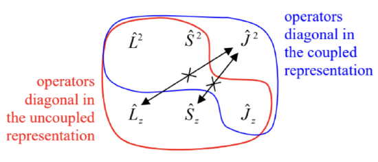Fig. 5.12. The Venn diagram of angular momentum operators, and their mutually-commuting groups.

This means that there are eigenstates shared by two operator groups encircled with colored lines in Fig. 12. The first group (encircled red), consists of all these operators but \(\hat{J}^{2}\). Hence there are eigenstates shared by the five remaining operators, and these states correspond to definite values of the corresponding quantum numbers: \(l, m_{l}, s, m_{s}\), and \(m_{j}\). Actually, only four of these numbers are independent, because due to Eq. (171) for these compatible operators, for each eigenstate of this group, their "magnetic" quantum numbers \(m\) have to satisfy the following relation: \[m_{j}=m_{l}+m_{s} .\] Hence the common eigenstates of the operators of this group are fully defined by just four quantum numbers, for example, \(l, m_{l}, s\), and \(m_{s}\). For some calculations, especially those for the systems whose Hamiltonians include only the operators of this group, it is convenient \({ }^{51}\) to use this set of eigenstates as the basis; frequently this approach is called the uncoupled representation.

However, in some situations we cannot ignore interactions between the orbital and spin degrees of freedom (in the common jargon, the spin-orbit coupling), which leads in particular to splitting (called the fine structure) of the atomic energy levels even in the absence of external magnetic field. I will discuss these effects in detail in the next chapter, and now will only note that they may be described by a term proportional to the product \(\hat{\mathbf{L}} \cdot \hat{\mathbf{S}}\), in the system’s Hamiltonian. If this term is substantial, the uncoupled representation becomes inconvenient. Indeed, writing \[\hat{J}^{2}=(\hat{\mathbf{L}}+\hat{\mathbf{S}})^{2}=\hat{L}^{2}+\hat{S}^{2}+2 \hat{\mathbf{L}} \cdot \hat{\mathbf{S}}, \quad \text { so that } 2 \hat{\mathbf{L}} \cdot \hat{\mathbf{S}}=\hat{J}^{2}-\hat{L}^{2}-\hat{S}^{2},\] and looking at Fig. 12 again, we see that operator \(\hat{\mathbf{L}} \cdot \hat{\mathbf{S}}\), describing the spin-orbit coupling, does not commute with operators \(\hat{L}_{z}\) and \(\hat{S}_{z}\). This means that stationary states of the system with such term in the Hamiltonian do not belong to the uncoupled representation’s basis. On the other hand, Eq. (181) shows that the operator \(\hat{\mathbf{L}} \cdot \hat{\mathbf{S}}\) does commute with all four operators of another group, encircled blue in Fig. 12. According to Eqs. (178), (179), and (181), all operators of that group also commute with each other, so that they have common eigenstates, described by the quantum numbers, \(l, s, j\), and \(m_{j}\). This group is the basis for the so-called coupled representation of particle states.

Excluding, for the notation briefness, the quantum numbers \(l\) and \(s\), common for both groups, it is convenient to denote the common ket-vectors of each group as, respectively,

Coupled and uncoupled bases

\[\ \begin{array}{ll}
\left|m_{l}, m_{s}\right\rangle, & \text { for the uncolpled representation's basis, } \\
\left|j, m_{j}\right\rangle, & \text { for the coupled representation's basis. }
\end{array}\]

As we will see in the next chapter, for the solution of some important problems (e.g., the fine structure of atomic spectra and the Zeeman effect), we will need the relation between the kets \(\left|j, m_{j}\right\rangle\) and the kets \(\left|m_{l}, m_{s}\right\rangle\). This relation may be represented as the usual linear superposition, \[\left|j, m_{j}\right\rangle=\sum_{m_{l}, m_{s}}\left|m_{l}, m_{s}\right\rangle\left\langle m_{l}, m_{s} \mid j, m_{j}\right\rangle .\] The short brackets in this relation, essentially the elements of the unitary matrix of the transformation between two eigenstate bases (182), are called the Clebsch-Gordan coefficients.

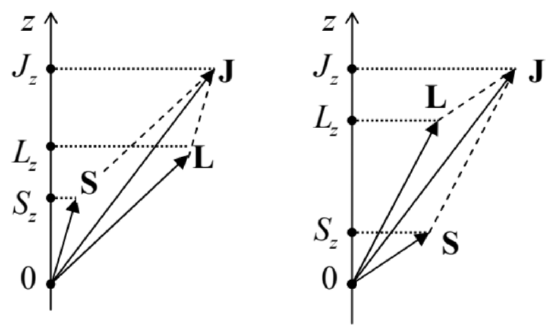
The best (though imperfect) classical interpretation of Eq. (183) I can offer is as follows. If the lengths of the vectors \(\mathbf{L}\) and \(\mathbf{S}\) (in quantum mechanics associated with the numbers \(l\) and \(s\), respectively), and also their scalar product \(\mathbf{L} \cdot \mathbf{S}\), are all fixed, then so is the length of the vector \(\mathbf{J}=\mathbf{L}+\mathbf{S}-\) whose length in quantum mechanics is described by the number \(j\). Hence, the classical image of a specific eigenket \(\left|j, m_{j}\right\rangle\), in which \(l, s, j\), and \(m_{j}\) are all fixed, is a state in which \(L^{2}, S^{2}, J^{2}\), and \(J_{z}\) are fixed. However, this fixation still allows for arbitrary rotation of the pair of vectors \(\mathbf{L}\) and \(\mathbf{S}\) (with a fixed angle between them, and hence fixed \(\mathbf{L} \cdot \mathbf{S}\) and \(J^{2}\) ) about the direction of the vector \(\mathbf{J}\) - see Fig. 13 .

Hence the components \(L_{z}\) and \(S_{z}\) in these conditions are not fixed, and in classical mechanics may take a continuum of values, two of which (with the largest and the smallest possible values of \(S_{z}\) ) are shown in Fig. 13. In quantum mechanics, these components are quantized, with their states represented by eigenkets \(\left|m_{l}, m_{s}\right\rangle\), so that a linear combination of such kets is necessary to represent a ket \(\left|j, m_{j}\right\rangle\). This is exactly what Eq. (183) does.

Fig. 5.13. A classical image of two different quantum states with the same quantum numbers \(l, s, j\), and \(m_{i}\), but different \(m_{l}\) and \(m_{s}\).

Some properties of the Clebsch-Gordan coefficients \(\left\langle m_{l}, m_{s} \mid j, m_{j}\right\rangle\) may be readily established. For example, the coefficients do not vanish only if the involved magnetic quantum numbers satisfy Eq. (180). In our current case, this relation is not an elementary corollary of Eq. (171), because in the Clebsch-Gordan coefficients, with the quantum numbers \(m_{l}, m_{s}\) in one state vector, and \(m_{j}\) in the other state vector, characterize the relation between different groups of the basis states, so we need to prove this fact. All matrix elements of the null-operator \[\hat{J}_{z}-\left(\hat{L}_{z}+\hat{S}_{z}\right)=\hat{0}\] should equal zero in any basis; in particular \[\left\langle j, m_{j}\left|\hat{J}_{z}-\left(\hat{L}_{z}+\hat{S}_{z}\right)\right| m_{l}, m_{s}\right\rangle=0 .\] Acting by the operator \(\hat{J}_{z}\) upon the bra-vector, and by the sum \(\left(\hat{L}_{z}+\hat{S}_{z}\right)\) upon the ket-vector, we get \[\left[m_{j}-\left(m_{l}+m_{s}\right)\right]\left\langle j, m_{j} \mid m_{l}, m_{s}\right\rangle=0,\] thus proving that \[\left\langle m_{l}, m_{s} \mid j, m_{s}\right\rangle \equiv\left\langle j, m_{s} \mid m_{l}, m_{s}\right\rangle^{*}=0, \quad \text { if } m_{j} \neq m_{l}+m_{s}\] For the most important case of spin-1/2 particles (with \(s=1 / 2\), and hence \(m_{s}=\pm 1 / 2\) ), whose uncoupled representation basis includes \(2 \times(2 l+1)\) states, the restriction (187) enables the representation of all non-zero Clebsch-Gordan coefficients on the simple "rectangular" diagram shown in Fig. \(14 .\) Indeed, each coupled-representation eigenket \(\left|j, m_{j}\right\rangle\), with \(m_{j}=m_{l}+m_{s}=m_{l} \pm 1 / 2\), may be related by nonzero Clebsch-Gordan coefficients to at most two uncoupled-representation eigenstates \(\left|m_{l}, m_{s}\right\rangle .\) Since \(m_{l}\) may only take integer values from \(-l\) to \(+l, m_{j}\) may only take semi-integer values on the interval \([-l-1 / 2\), \(l+1 / 2]\). Hence, by the definition of \(j\) as \(\left(m_{j}\right)_{\max }\), its maximum value has to be \(l+1 / 2\), and for \(m_{j}=l+1 / 2\), this is the only possible value with this \(j\). This means that the uncoupled state with \(m_{l}=l\) and \(m_{s}=1 / 2\) should be identical to the coupled-representation state with \(j=l+1 / 2\) and \(m_{j}=l+1 / 2\) : \[\left|j=l+1 / 2, m_{j}=l+1 / 2\right\rangle=\left|m_{l}=m_{j}-1 / 2, m_{s}=+1 / 2\right\rangle .\] In Fig. 14, these two identical states are represented with the top-rightmost point (the uncoupled representation) and the sloped line passing through it (the coupled representation).

Fig. 5.14. A graphical representation of possible basis states of a spin- \(1 / 2\) particle with a fixed \(l\). Each dot corresponds to an uncoupled-representation ket-vector \(\left|m_{l}, m_{s}\right\rangle\), while each sloped line corresponds to one coupled-representation ket-vector \(\left|j, m_{j}\right\rangle\), related by Eq. (183) to the kets \(\left|m_{l}, m_{s}\right\rangle\) whose dots it connects.

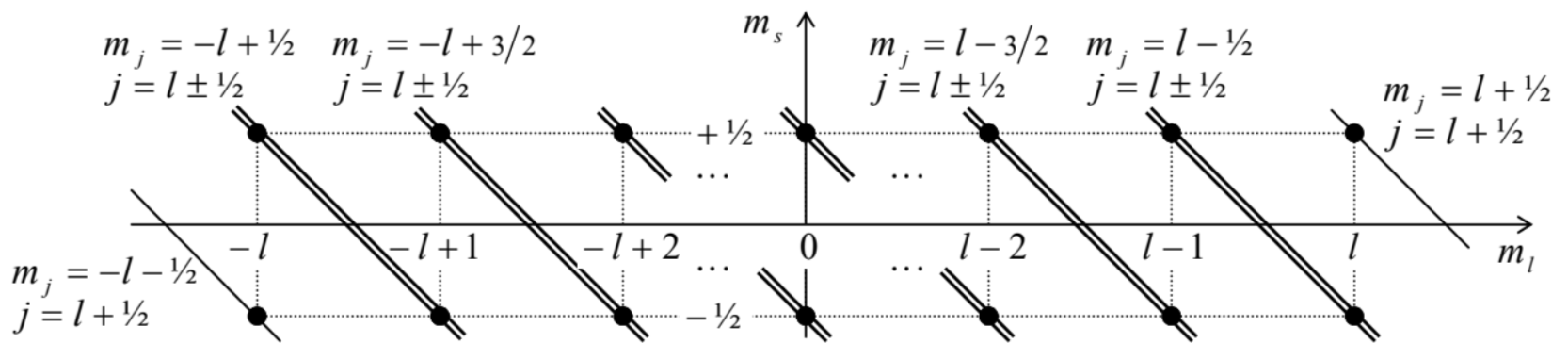
However, already the next value of this quantum number, \(m_{j}=l-1 / 2\), is compatible with two values of \(j\), so that each \(\left|m_{l}, m_{s}\right\rangle\) ket has to be related to two \(\left|j, m_{j}\right\rangle\) kets by two Clebsch-Gordan coefficients. Since \(j\) changes in unit steps, these values of \(j\) have to be \(l \pm 1 / 2\). This choice, \[j=l \pm 1 / 2,\] evidently satisfies all lower values of \(m_{j}\) as well - see Fig. 14. \({ }^{52}\) (Again, only one value, \(j=l+1 / 2\), is necessary to represent the state with the lowest \(m_{j}=-l-1 / 2-\) see the bottom-leftmost point of that diagram.) Note that the total number of the coupled-representation states is \(1+2 \times 2 l+1 \equiv 2(2 l+1)\), i.e. is the same as those in the uncoupled representation. So, for spin- \(-\frac{1}{2}\) systems, each sum (183), for fixed \(j\) and \(m_{j}\) (plus the fixed common parameter \(l\), plus the common \(s=1 / 2\) ), has at most two terms, i.e. involves at most two Clebsch-Gordan coefficients.

These coefficients may be calculated in a few steps, all but the last one rather simple even for an arbitrary spin \(s\). First, the similarity of the vector operators \(\hat{\mathbf{J}}\) and \(\hat{\mathbf{S}}\) to the operator \(\hat{\mathbf{L}}\), expressed by Eqs. (169), (175), and (177), may be used to argue that the matrix elements of the operators \(\hat{S}_{\pm}\)and \(\hat{J}_{\pm}\), defined similarly to \(\hat{L}_{\pm}\), have the matrix elements similar to those given by Eq. (164). Next, acting by the operator \(\hat{J}_{\pm}=\hat{L}_{\pm}+\hat{S}_{\pm}\)upon both parts of Eq. (183), and then inner-multiplying the result by the bra vector \(\left\langle m_{l}, m_{s}\right|\) and using the above matrix elements, we may get recurrence relations for the ClebschGordan coefficients with adjacent values of \(m_{l}, m_{s}\), and \(m_{j}\). Finally, these relations may be sequentially applied to the adjacent states in both representations, starting from any of the two states common for them - for example, from the state with the ket-vector (188), corresponding to the top right point in Fig. \(14 .\)

Let me leave these straightforward but a bit tedious calculations for the reader’s exercise, and just cite the final result of this procedure for \(s=1 / 2: 53\) \[\begin{aligned} &\left\langle m_{l}=m_{j}-1 / 2, m_{s}=+1 / 2 \mid j=l \pm 1 / 2, m_{j}\right\rangle=\pm\left(\frac{l \pm m_{j}+1 / 2}{2 l+1}\right)^{1 / 2}, \\ &\left\langle m_{l}=m_{j}+1 / 2, m_{s}=-1 / 2 \mid j=l \pm 1 / 2, m_{j}\right\rangle=+\left(\frac{l \mp m_{j}+1 / 2}{2 l+1}\right)^{1 / 2} . \end{aligned}\] In this course, these relations will be used mostly in Sec. \(6.4\) for an analysis of the anomalous Zeeman effect. Moreover, the angular momentum addition theory described above is also valid for the addition of angular momenta of multiparticle system components, so we will revisit it in Chapter 8 .

To conclude this section, I have to note that the Clebsch-Gordan coefficients (for arbitrary \(s\) ) participate also in the so-called Wigner-Eckart theorem that expresses the matrix elements of spherical tensor operators, in the coupled-representation basis \(\left|j, m_{j}\right\rangle\), via a reduced set of matrix elements. This theorem may be useful, for example, for the calculation of the rate of quantum transitions to/from high- \(n\) states in spherically-symmetric potentials. Unfortunately, a discussion of this theorem and its applications would require a higher mathematical background than I can expect from my readers, and more time/space than I can afford. \({ }^{54}\)

---

\({ }^{49}\) As a reminder, in the Standard Model of particle physics, such hadrons as mesons and baryons (notably including protons and neutrons) are essentially composite particles. However, at non-relativistic energies, protons and neutrons may be considered fundamental particles with \(s=1 / 2\).

\({ }^{50}\) Let me hope that the difference between the quantum number \(j\), and the indices \(j, j^{\prime}, j\) " numbering the Cartesian components in the relations like Eqs. (168) or (174), is absolutely clear from the context.

\({ }^{51}\) This is especially true for motion in spherically-symmetric potentials, whose stationary states correspond to definite \(l\) and \(m_{l}\); however, the relations discussed in this section are important for some other problems as well.

\({ }^{52}\) Eq. (5.189) allows a semi-qualitative classical interpretation in terms of the vector diagrams shown in Fig. 13: since, according to Eq. (169), \(\hbar s\) gives the scale of the length of the vector \(\mathbf{S}\), if it is small \((s=1 / 2)\), the length of vector \(\mathbf{J}\) (similarly scaled by \(\hbar j\) ) cannot deviate much from the length of the vector \(\mathbf{L}\) (scaled by \(\hbar l\) ) for any spatial orientation of these vectors, so that \(j\) cannot differ from \(l\) too much. Note also that for a fixed \(m_{j}\), the alternating sign in Eq. (189) is independent of the sign of \(m_{s}-\) see also Eqs. (190).

\({ }^{53}\) For arbitrary spin \(s\), the calculations and even the final expressions for the Clebsch-Gordan coefficients are rather bulky. They may be found, typically in a table form, mostly in special monographs - see, e.g., A. Edmonds, Angular Momentum in Quantum Mechanics, Princeton U. Press, \(1957 .\)

\({ }^{54}\) For the interested reader, I can recommend either Sec. \(17.7\) in E. Merzbacher, Quantum Mechanics, \(3^{\text {rd }}\) ed., Wiley, 1998, or Sec. \(3.10\) in J. Sakurai, Modern Quantum Mechanics, Addison-Wesley, \(1994 .\)