6.4: The Zeeman Effect

Now, we are ready to review the Zeeman effect - the atomic level splitting by an external magnetic field. \({ }^{17}\) Using Eq. (3.26), with \(q=-e\), for the description of the electron’s orbital motion in the field, and the Pauli Hamiltonian (4.163), with \(\gamma=-e / m_{\mathrm{e}}\), for the electron spin’s interaction with the field, we see that even for a hydrogen-like (i.e. single-electron) atom/ion, neglecting the relativistic effects, the full Hamiltonian is rather involved: \[\hat{H}=\frac{1}{2 m_{\mathrm{e}}}(\hat{\mathbf{p}}+e \hat{\mathbf{A}})^{2}-\frac{Z e^{2}}{4 \pi \varepsilon_{0} r}+\frac{e}{m_{\mathrm{e}}} \mathscr{B} \cdot \hat{\mathbf{S}}\]

There are several simplifications we may make. First, let us assume that the external field is spatial-uniform on the atomic scale (which is a very good approximation for most cases), so that we can take its vector potential in an axially-symmetric gauge - cf. Eq. (3.132): \[\mathbf{A}=\frac{1}{2} \mathscr{B} \times \mathbf{r} .\] Second, let us neglect the terms proportional to \(\mathscr{B}^{2}\), which are small in practical magnetic fields of the order of a few teslas. \({ }^{18}\) The remaining term in the effective kinetic energy, describing the interaction with the magnetic field, is linear in the momentum operator, so that we may repeat the standard classical calculation \({ }^{19}\) to reduce it to the product of \(\mathscr{B}\) by the orbital magnetic moment’s component \(m_{z}=-\) \(e L_{z} / 2 m_{\mathrm{e}}\) - besides that both \(m_{z}\) and \(L_{z}\) should be understood as operators now. As a result, the Hamiltonian (63) reduces to Eq. (1), \(\hat{H}^{(0)}+\hat{H}^{(1)}\), where \(\hat{H}^{(0)}\) is that of the atom at \(\mathscr{B}=0\), and \[\hat{H}^{(1)}=\frac{e \mathscr{R}}{2 m_{\mathrm{e}}}\left(\hat{L}_{z}+2 \hat{S}_{z}\right)\] This expression immediately reveals the major complication with the Zeeman effect’s analysis. Namely, in comparison with the equal orbital and spin contributions to the total angular momentum (5.170) of the electron, its spin produces a twice larger contribution to the magnetic moment, so that the right-hand side of Eq. (65) is not proportional to the total angular moment \(\mathbf{J}\). As a result, the effect’s description is simple only in two limits.

If the magnetic field is so high that its effects are much stronger than the relativistic (finestructure) effects discussed in the previous section, we may treat the two terms in Eq. (65) as independent perturbations of different (orbital and spin) degrees of freedom. Since each of the perturbation matrices is diagonal in its own \(z\)-basis, we can again use Eq. (27) to write \[E-E^{(0)}=\frac{e \mathscr{B}}{2 m_{\mathrm{e}}}\left(\left\langle n, l, m_{l}\left|\hat{L}_{z}\right| n, l, m_{l}\right\rangle+2\left\langle m_{s}\left|\hat{S}_{z}\right| m_{s}\right\rangle\right)=\frac{e \mathscr{B}}{2 m_{\mathrm{e}}}\left(\hbar m_{l}+2 \hbar m_{s}\right)=\mu_{\mathrm{B}} \mathscr{B}\left(m_{l} \pm 1\right) .\] This result describes splitting of each \(2 \times(2 l+1)\)-degenerate energy level, with certain \(n\) and \(l\), into ( \(2 l\) +3) levels (Fig. 5), with the adjacent level distance of \(\mu_{\mathrm{B}} \mathscr{B}\), of the order of \(10^{-4} \mathrm{eV}\) per tesla.

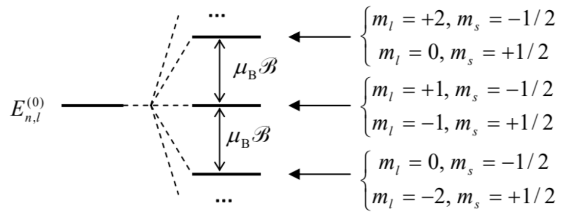Fig. 6.5. The Paschen-Back effect.

Note that all the levels, these besides the top and bottom ones, remain doubly degenerate. This limit of the Zeeman effect is sometimes called the Paschen-Back effect - whose simplicity was recognized only in the \(1920 \mathrm{~s}\), due to the need in very high magnetic fields for its observation.

In the opposite limit of relatively low magnetic fields, the Zeeman effect takes place on the background of the much larger fine-structure splitting. As was discussed in Sec. 3, at \(\mathscr{R}=0\) each split sub-level has a \(2 \times(2 j+1)\)-fold degeneracy corresponding to \((2 j+1)\) different values of the half-integer quantum number \(m_{j}\), ranging from \(-j\) to \(+j\), and two values of the integer \(l=j \mp 1 / 2-\) see Fig. \(4 .^{20}\) The magnetic field lifts this degeneracy. Indeed, in the coupled representation discussed in Sec. 5.7, the perturbation (65) is described by the matrix with elements \[\begin{aligned} H^{(1)} &=\frac{e \mathscr{B}}{2 m_{\mathrm{e}}}\left\langle j, m_{j}\left|\hat{L}_{z}+2 \hat{S}_{z}\right| j^{\prime}, m_{j^{\prime}}\right\rangle \equiv \frac{e \mathscr{B}}{2 m_{\mathrm{e}}}\left\langle j, m_{j}\left|\hat{J}_{z}+\hat{S}_{z}\right| j^{\prime}, m_{j^{\prime}}\right\rangle \\ &=\frac{e \mathscr{B}}{2 m_{\mathrm{e}}}\left(\hbar m_{j} \delta_{m_{j} m_{j^{\prime}}}+\left\langle j, m_{j}\left|\hat{S}_{z}\right| j^{\prime}, m_{j^{\prime}}\right\rangle\right) . \end{aligned}\] To spell out the second term, let us use the general expansion (5.183) for the particular case \(s=\) \(1 / 2\), when (as was discussed in the end of Sec. 5.7) it has at most two non-vanishing terms, with the Clebsh-Gordan coefficients (5.190): \[\begin{aligned} &\left|j=l \pm 1 / 2, m_{j}\right\rangle \\ &=\pm\left(\frac{l \pm m_{j}+1 / 2}{2 l+1}\right)^{1 / 2}\left|m_{l}=m_{j}-1 / 2, m_{s}=+1 / 2\right\rangle+\left(\frac{l \mp m_{j}+1 / 2}{2 l+1}\right)^{1 / 2}\left|m_{l}=m_{j}+1 / 2, m_{s}=-1 / 2\right\rangle . \end{aligned}\] Taking into account that the operator \(\hat{S}_{z}\) gives non-zero brackets only for \(m_{s}=m_{s^{\prime}}\), the \(2 \times 2\) matrix of elements \(\left\langle m_{l}=m_{j} \pm 1 / 2, m_{\mathrm{s}}=\mp 1 / 2\left|\hat{S}_{z}\right| m_{l}=m_{j} \pm 1 / 2, m_{\mathrm{s}}=\mp 1 / 2\right\rangle\) is diagonal, so we may use Eq. (27) to get \[\begin{aligned} E-E^{(0)} &=\frac{e \mathscr{R}}{2 m_{\mathrm{e}}}\left[\hbar m_{j}+\frac{\hbar}{2} \frac{\left(l \pm m_{j}+1 / 2\right)}{2 l+1}-\frac{\hbar}{2} \frac{\left(l \mp m_{j}+1 / 2\right)}{2 l+1}\right] \\ & \equiv \frac{e \mathscr{B}}{2 m_{\mathrm{e}}} \hbar m_{j}\left(1 \pm \frac{1}{2 l+1}\right) \equiv \mu_{\mathrm{B}} \mathscr{R} m_{j}\left(1 \pm \frac{1}{2 l+1}\right), \quad \text { for }-j \leq m_{j} \leq+j \end{aligned}\] where the two signs correspond to the two possible values of \(l=j \mp 1 / 2-\) see Fig. 6 .

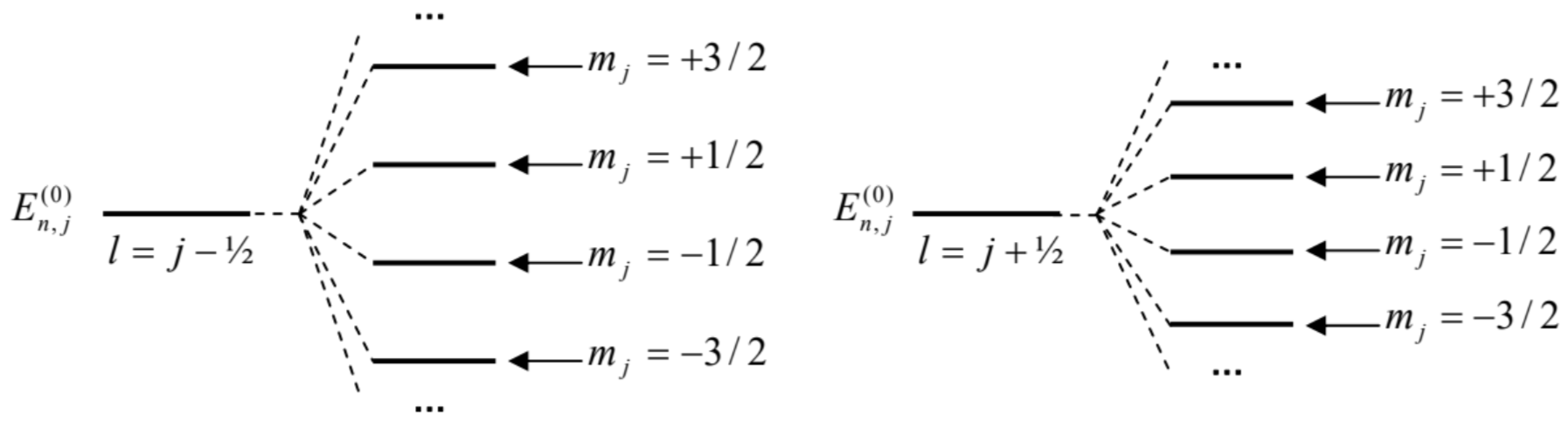Fig. 6.6. The anomalous Zeeman effect in a hydrogen-like atom/ion.

We see that the magnetic field splits each sub-level of the fine structure, with a given \(l\), into \(2 j+\) 1 equidistant levels, with the distance between the levels depending on \(l\). In the late \(1890 \mathrm{~s}\), when the Zeeman effect was first observed, there was no notion of spin at all, so that this puzzling result was called the anomalous Zeeman effect. (In this terminology, the normal Zeeman effect is the one with no spin splitting, i.e. without the second terms in the parentheses of Eqs. (66), (67), and (69); it was first observed in 1898 by Preston Thomas in atoms with zero net spin.)

The strict quantum-mechanical analysis of the anomalous Zeeman effect for arbitrary \(s\) (which is important for applications to multi-electron atoms) is conceptually not complex, but requires explicit expressions for the corresponding Clebsch-Gordan coefficients, which are rather bulky. Let me just cite the unexpectedly simple result of this analysis: \[\Delta E=\mu_{\mathrm{B}} \mathscr{M} m_{j} g,\] where \(g\) is the so-called Lande factor:²¹ \[g=1+\frac{j(j+1)+s(s+1)-l(l+1)}{2 j(j+1)}\]

For \(s=1 / 2\) (and hence \(j=l \pm 1 / 2\) ), this factor is reduced to the parentheses in the last forms of Eq. (69).

It is remarkable that Eqs. (70) may be readily derived using very plausible classical arguments, similar to those used in Sec. \(5.7\) - see Fig. \(5.13\) and its discussion. As was discussed in Sec. 5.6, in the absence of spin, the quantization of the observable \(L_{z}\) is an extension of the classical picture of the torque-induced precession of the vector \(\mathbf{L}\) about the magnetic field’s direction, so that the interaction energy, proportional to \(\mathscr{R} L_{z}=\mathscr{B} \cdot \mathbf{L}\), remains constant \(-\) see Fig. \(7 \mathrm{a}\). On the other hand, at the spin-orbit interaction without an external magnetic field, the Hamiltonian function of the system includes the product S.L, so that in the stationary state it has to be constant, together with \(J^{2}, L^{2}\), and \(S^{2} .\) Hence, this system’s classical image is a joint precession of the vectors \(\mathbf{S}\) and \(\mathbf{L}\) about the direction of the vector \(\mathbf{J}=\) \(\mathbf{L}+\mathbf{S}\), in such a manner that the spin-orbit interaction energy, proportional to the product \(\mathbf{L} \cdot \mathbf{S}\), remains constant (Fig. \(7 \mathrm{~b}\) ). On this backdrop, the anomalous Zeeman effect in a relatively weak magnetic field \(\mathscr{B}\) \(=\mathscr{R} \mathbf{n}_{z}\) corresponds to a much slower precession of the vector \(\mathbf{J}\) about the \(z\)-axis, "dragging" with it the vectors \(\mathbf{L}\) and \(\mathbf{S}\), rapidly rotating around it.

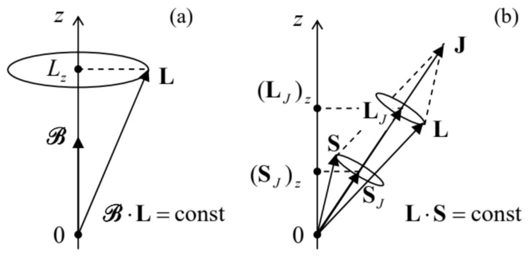Fig. 6.7. Classical images of (a) the orbital angular momentum’s quantization in a magnetic field, and (b) the fine-structure level splitting.

This physical picture allows us to conjecture that what is important for the slow precession rate are only the vectors \(\mathbf{L}\) and \(\mathbf{S}\) averaged over the period of their much faster precession around vector \(\mathbf{J}-\) in other words, only their components \(\mathbf{L}_{J}\) and \(\mathbf{S}_{J}\) along the vector \(\mathbf{J}\). Classically, these components may be calculated as \[\mathbf{L}_{J}=\frac{\mathbf{L} \cdot \mathbf{J}}{J^{2}} \mathbf{J}, \quad \text { and } \mathbf{S}_{J}=\frac{\mathbf{S} \cdot \mathbf{J}}{J^{2}} \mathbf{J} .\] The scalar products participating in these expressions may be readily expressed via the squared lengths of the vectors, using the following geometric formulas: \[S^{2}=(\mathbf{J}-\mathbf{L})^{2} \equiv J^{2}+L^{2}-2 \mathbf{L} \cdot \mathbf{J}, \quad L^{2}=(\mathbf{J}-\mathbf{S})^{2} \equiv J^{2}+S^{2}-2 \mathbf{J} \cdot \mathbf{S} .\] As a result, we get the following time average: \[\begin{aligned} \overline{L_{z}+2 S_{z}} &=\left(\mathbf{L}_{J}+2 \mathbf{S}_{J}\right)_{z}=\left(\frac{\mathbf{L} \cdot \mathbf{J}}{J^{2}} \mathbf{J}+2 \frac{\mathbf{S} \cdot \mathbf{J}}{J^{2}} \mathbf{J}\right)_{z}=\frac{J_{z}}{J^{2}}(\mathbf{L} \cdot \mathbf{J}+2 \mathbf{S} \cdot \mathbf{J}) \\ &=J_{z} \frac{\left(J^{2}+L^{2}-S^{2}\right)+2\left(J^{2}+S^{2}-L^{2}\right)}{2 J^{2}} \equiv J_{z}\left(1+\frac{J^{2}+S^{2}-L^{2}}{2 J^{2}}\right) . \end{aligned}\] The last move is to smuggle in some quantum mechanics by using, instead of the vector lengths squared and the \(z\)-component of \(J_{z}\), their eigenvalues given by Eqs. (5.169), (5.175), and (5.177). As a result, we immediately arrive at the exact Eqs. (70). This coincidence encourages thinking about quantum mechanics of angular momenta in the classical terms of torque-induced precession, which turns out to be very fruitful in some more complex problems of atomic and molecular physics.

The high-field limit and low-field limits of the Zeeman effect, described respectively by Eqs. (66) and (69), are separated by a medium field range, in which the Zeeman splitting is of the order of the fine-structure splitting analyzed in \(\mathrm{Sec}\). 3. There is no time in this course for a quantitative analysis of this crossover. \({ }^{22}\)

---

\({ }^{17}\) It was discovered experimentally in 1896 by Pieter Zeeman who, amazingly, was fired from the University of Leiden for unauthorized use of lab equipment for this work - just to receive a Nobel Prize for it in a few years!

\({ }^{18}\) Despite its smallness, the quadratic term is necessary for a description of the negative contribution of the orbital motion to the magnetic susceptibility \(\chi_{\mathrm{m}}\) (the so-called orbital diamagnetism, see EM Sec. 5.5), whose analysis, using Eq. (63), is left for the reader’s exercise.

\({ }^{19}\) See, e.g., EM Sec. 5.4, in particular Eqs. (5.95) and (5.100).

\({ }^{20}\) In the almost-hydrogen-like, but more complex atoms (such as those of alkali metals), the degeneracy in \(l\) may be lifted by electron-electron Coulomb interaction even in the absence of external magnetic field.

\({ }^{21}\) This formula is frequently used with capital letters \(J, S\), and \(L\), which denote the quantum numbers of the atom as a whole.

\({ }^{22}\) For a more complete discussion of the Stark, Zeeman, and fine-structure effects in atoms, I can recommend, for example, either the monograph by G. Woolgate cited above, or the one by I. Sobelman, Theory of Atomic Spectra, Alpha Science, \(2006 .\)