6.7: Golden Rule for Step-like Perturbations

Now let us reuse some of our results for a perturbation being turned on at \(t=0\), but after that time-independent: \[\hat{H}^{(1)}(t)= \begin{cases}0, & \text { for } t<0 \\ \hat{H}=\mathrm{const}, & \text { for } t \geq 0\end{cases}\] A superficial comparison of this equality and the former Eq. (86) seems to indicate that we may use all our previous results, taking \(\omega=0\) and replacing \(\hat{A}+\hat{A}^{\dagger}\) with \(\hat{H}^{(1)}\). However, that conclusion (which would give us a wrong factor of 2 in the result) does not take into account the fact that analyzing both the two-level approximation in Sec. 5 , and the Golden Rule in Sec. 6 , we have dropped the second (nonresonant) term in Eq. (90). In our current case (134), with \(\omega=0\), there is no such difference between these terms. This why it is more prudent to use the general Eq. (84), \[i \hbar \dot{a}_{n}=\sum_{n^{\prime}} a_{n^{\prime}} H_{n n^{\prime}} e^{i \omega_{n n^{\prime}}},\] in which the matrix element of the perturbation is now time-independent at \(t>0\). We see that it is formally equivalent to Eq. (88) with only the first (resonant) term kept, if we make the following replacements: \[\hat{A} \rightarrow \hat{H}, \quad \Delta_{n n^{\prime}} \equiv \omega-\omega_{n n^{\prime}} \rightarrow-\omega_{n n^{\prime}} .\] Let us use this equivalency to consider the results of coupling between a discrete-energy state \(n\) ’, into which the particle is initially placed, and a dense group of states with a quasi-continuum spectrum, in the same energy range. Figure 11 a shows an example of such a system: a particle is initially (say, at \(t\) \(=0\) ) placed into a potential well separated by a penetrable potential barrier from a formally infinite region with a continuous energy spectrum. Let me hope that the physical discussion in the last section makes the outcome of such an experiment evident: the particle will gradually and irreversibly tunnel out of the well, so that the probability \(W_{n} \cdot(t)\) of its still residing in the well will decay in accordance with Eq. (114). The rate of this decay may be found by making the replacements (136) in Eq. (111): \[\Gamma=\frac{2 \pi}{\hbar}\left|H_{n n^{\prime}}\right|^{2} \rho_{n},\] where the states \(n\) and \(n\) ’ now have virtually the same energy. \({ }^{42}\)

Fig. 6.11. Tunneling from a discrete-energy state \(n\) ’: (a) to a state continuum, and (b) to another discrete-energy state \(n\).

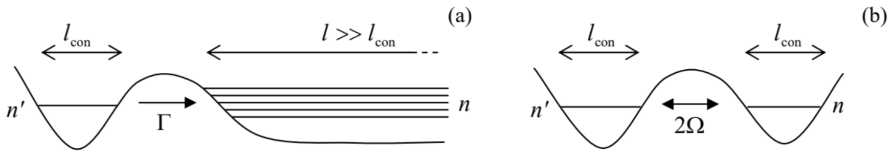
It is very informative to compare this result, semi-quantitatively, with Eq. (105) for a symmetric \(\left(E_{n}=E_{n}\right.\) ) system of two potential wells separated by a similar potential barrier-see Fig. 11b. For the symmetric case, i.e. \(\xi=0\), Eq. (105) is reduced to simply \[\Omega=\frac{1}{\hbar}\left|H_{n n^{\prime}}\right|_{\mathrm{con}} .\] Here I have used the index "con" (from "confinement") to emphasize that this matrix element is somewhat different from the one participating in Eq. (137), even if the potential barriers are similar. Indeed, in the latter case, the matrix element, \[H_{n n^{\prime}}=\left\langle n|\hat{H}| n^{\prime}\right\rangle=\int \psi_{n^{\prime}}^{*} \hat{H} \psi_{n} d x,\] has to be calculated for two wavefunctions \(\psi_{n}\) and \(\psi_{n}\) ’ confined to spatial intervals of the same scale \(l_{\text {con }}\), while in Eq. (137), the wavefunctions \(\psi_{n}\) are extended over a much larger distance \(l>>l_{\text {con }}-\operatorname{see}\) Fig. 11. As Eq. (128) tells us, in the 1D model this means an additional small factor of the order of \(\left(l_{\text {con }} / l\right)^{1 / 2} .\) Now using Eq. (128) as a crude but suitable model for the final-state wavefunctions, we arrive at the following estimate, independent of the artificially introduced length \(l\) : \[\hbar \Gamma \sim 2 \pi\left|H_{n n^{\prime}}\right|_{\mathrm{con}}^{2} \frac{l_{\mathrm{con}}}{l} \rho_{n} \sim 2 \pi\left|H_{n n^{\prime}}\right|_{\mathrm{con}}^{2} \frac{l_{\mathrm{con}}}{l} \frac{l m}{2 \pi \hbar^{2} k_{n}} \sim \frac{\left|H_{n n^{\prime}}\right|_{\mathrm{con}}^{2}}{\Delta E_{n^{\prime}}} \equiv \frac{(\hbar \Omega)^{2}}{\Delta E_{n^{\prime}}}\] where \(\Delta E_{n} \sim \hbar^{2} / m l_{\text {con }}^{2}\) is the scale of the differences between the eigenenergies of the particle in an unperturbed potential well. Since the condition of validity of Eq. (138) is \(\hbar \Omega<<\Delta E_{n}\), we see that

\[\hbar \Gamma \sim \frac{\hbar \Omega}{\Delta E_{n}} \hbar \Omega<<\hbar \Omega . .\] This (sufficiently general \({ }^{43}\) ) perturbative result confirms the conclusion of a more particular analysis carried out in the end of Sec. 2.6: the rate of the (irreversible) quantum tunneling into a state continuum is always much lower than the frequency of (reversible) quantum oscillations between discrete states separated with the same potential barrier - at least for the case when both are much lower than \(\Delta E_{n} / \hbar\), so that the perturbation theory is valid. A very handwaving interpretation of this result is that the particle oscillates between the confined state in the well and the space-extended states behind the barrier many times before finally "deciding to perform" an irreversible transition into the unconfined continuum. This qualitative picture is consistent with experimentally observable effects of dispersive electromagnetic environments on electron tunneling. \({ }^{44}\)

Let me conclude this section (and this chapter) with the application of Eq. (137) to a very important case, which will provide a smooth transition to the next chapter’s topic. Consider a composite system consisting of two component systems, \(a\) and \(b\), with the energy spectra sketched in Fig. 12 .

Fig. 6.12. Energy relaxation in system a due to its weak coupling to system \(\ b\) (which serves as the environment of \(\ a\)).

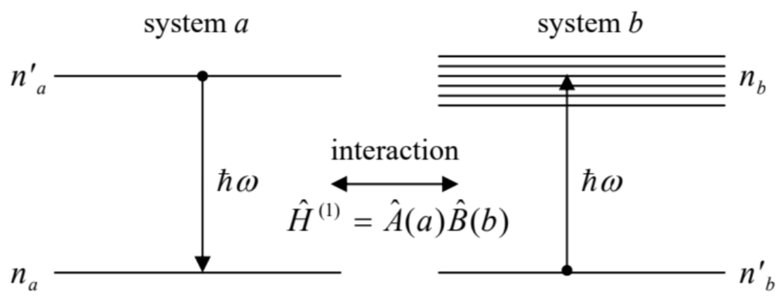
Let the systems be completely independent initially. The independence means that in the absence of their coupling, the total Hamiltonian of the system may be represented as a sum of two operators: \[\hat{H}^{(0)}=\hat{H}_{a}(a)+\hat{H}_{b}(b),\] where the arguments \(a\) and \(b\) symbolize the non-overlapping sets of the degrees of freedom of the two systems. Such operators, belonging to their individual, different Hilbert spaces, naturally commute. Similarly, the eigenkets of the system may be naturally factored as \[|n\rangle=\left|n_{a}\right\rangle \otimes\left|n_{b}\right\rangle .\] The direct product \(\operatorname{sign} \otimes\) is used here (and below) to denote the formation of a joint ket-vector from the kets of the independent systems, belonging to different Hilbert spaces. Evidently, the order of operands in such a product may be changed at will. As a result, its eigenenergies separate into a sum, just as the Hamiltonian (142) does: \[\hat{H}^{(0)}|n\rangle=\left(\hat{H}_{a}+\hat{H}_{b}\right)\left|n_{a}\right\rangle \otimes\left|n_{b}\right\rangle \equiv\left(\hat{H}_{a}\left|n_{a}\right\rangle\right) \otimes\left|n_{b}\right\rangle+\left(\hat{H}_{b}\left|n_{b}\right\rangle\right) \otimes\left|n_{a}\right\rangle=\left(E_{n a}+E_{n b}\right)|n\rangle .\] In such composite systems, the relatively weak interaction of its components may be usually represented as a bilinear product of two Hermitian operators, each depending only on the degrees of freedom of one component system: \[\hat{H}^{(1)}=\hat{A}(a) \hat{B}(b) .\] A very common example of such an interaction is the electric-dipole interaction between an atomicscale system (with a linear size of the order of the Bohr radius \(r_{\mathrm{B}} \sim 10^{-10} \mathrm{~m}\) ) and the electromagnetic field at optical frequencies \(\omega \sim 10^{16} \mathrm{~s}^{-1}\), with the wavelength \(\lambda=2 \pi c / \omega \sim 10^{-6} \mathrm{~m} \gg r_{\mathrm{B}}:{ }^{45}\) \[\hat{H}^{(1)}=-\hat{\mathbf{d}} \cdot \hat{E}, \quad \text { with } \hat{\mathbf{d}} \equiv \sum_{k} q_{k} \hat{\mathbf{r}}_{k},\] where the dipole electric moment \(\mathbf{d}\) depends only on the positions \(\mathbf{r}_{k}\) of the charged particles (numbered with index \(k\) ) of the atomic system, while that of electric field \(\mathscr{E}\) is a function of only the electromagnetic field’s degrees of freedom - to be discussed in Chapter 9 below.

Returning to the general situation shown in Fig. 12, if the component system \(a\) was initially in an excited state \(n_{a}^{\prime}\), the interaction (145), turned on at some moment of time, may bring it into another discrete state \(n_{a}\) of a lower energy - for example, the ground state. In the process of this transition, the released energy, in the form of an energy quantum \[\hbar \omega \equiv E_{n^{\prime} a}-E_{n a},\] is picked up by the system \(b\) : \[E_{n b}=E_{n^{\prime} b}+\hbar \omega \equiv E_{n^{\prime} b}+\left(E_{n^{\prime} a}-E_{n a}\right),\] so that the total energy \(E=E_{a}+E_{b}\) of the system does not change. (If the states \(n_{a}\) and \(n_{b}^{\prime}\) are the ground states of the two component systems, as they are in most applications of this analysis, and we take the ground state energy \(E_{\mathrm{g}}=E_{n a}+E_{n^{\prime} b}\) of the composite system for the reference, then Eq. (148) gives merely \(E_{n b}=E_{n^{\prime} a}\).) If the final state \(n_{b}\) of the system \(b\) is inside a state group with a quasi-continuous energy spectrum (Fig. 12), the process has the exponential character (114) \(4^{4}\) and may be interpreted as the effect of energy relaxation of the system \(a\), with the released energy quantum \(\hbar \omega\) absorbed by the system \(b\). Note that since the quasi-continuous spectrum essentially requires a system of large spatial size, such a model is very convenient for description of the environment \(b\) of the quantum system \(a\). (In physics, the "environment" typically means all the Universe - less the system under consideration.)

If the relaxation rate \(\Gamma\) is sufficiently low, it may be described by the Golden Rule (137). Since the perturbation (145) does not depend on time explicitly, and the total energy \(E\) does not change, this relation, with the account of Eqs. (143) and (145), takes the form \[\Gamma=\frac{2 \pi}{\hbar}\left|A_{n n^{\prime}}\right|^{2}\left|B_{n n^{\prime}}\right|^{2} \rho_{n}, \quad \text { where } A_{n n^{\prime}} \equiv\left\langle n_{a}|\hat{A}| n_{a}^{\prime}\right\rangle, \quad \text { and } B_{n n^{\prime}}=\left\langle n_{b}|\hat{B}| n_{b}^{\prime}\right\rangle,\] where \(\rho_{n}\) is the density of the final states of the system \(b\) at the relevant energy (147). In particular, Eq. (149), with the dipole Hamiltonian (146), enables a very straightforward calculation of the natural linewidth of atomic electric-dipole transitions. However, such calculation has to be postponed until Chapter 9, in which we will discuss the electromagnetic field quantization - i.e., the exact nature of the states \(n_{b}\) and \(n_{b}\) for this problem, and hence will be able to calculate \(B_{n n^{\prime}}\) and \(\rho_{n}\). Instead, I will now proceed to a general discussion of the effects of quantum systems interaction with their environment, toward which the situation shown in Fig. 12 provides a clear conceptual path.

---

\({ }^{42}\) The condition of validity of Eq. (137) is again given by Eq. (117), just with \(\omega=0\) in the upper limit for \(\Gamma\).

\({ }^{43}\) It is straightforward to verify that the estimate (141) is valid for similar problems of any spatial dimensionality, not just for the 1D case we have analyzed.

\({ }^{44}\) See, e.g., P. Delsing et al., Phys. Rev. Lett. 63, 1180 (1989).

\({ }^{45}\) See, e.g., EM Sec. 3.1, in particular Eq. (3.16), in which letter \(\mathbf{p}\) is used for the electric dipole moment.

\({ }^{46}\) Such process is spontaneous: it does not require any external agent, and starts as soon as either the interaction (145) has been turned on, or (if it is always on) as soon as the system \(a\) is placed into the excited state \(n_{a}^{\prime}\).