
6: Many-body problems, systems of identical particles
- Page ID
- 50558

So far we have considered single particle problems, a particle moving in a given potential. In the model of the H atom considered previously the potential was given apriori by the Coulomb field of the proton. In a physical system, however, one has usually several particles that interact with each other. In reality already the H atom consists of two particles: a proton which is the nucleus and the electron.
Chapters 2, 4 and 5. The two-body problem in classical mechanics.
Entanglement of two particles
In order to see the peculiarities of the situation, we shall consider, as an example, the case of the H atom as a two-body problem. The wave function of such a system should depend on the coordinates of the electron \(\mathbf{r}_{e}\) as well as on the coordinates of the proton \(\mathbf{R}_{n}\), where n refers to the nucleus. The Hamiltonian of this two particle system is
\(H_{n e}=\frac{\mathbf{P}_{n}^{2}}{2 M_{n}}+\frac{\mathbf{P}_{e}^{2}}{2 m_{e}}-\frac{e_{0}^{2}}{\left|\mathbf{R}_{n}-\mathbf{r}_{e}\right|}\) (6.1)
and the wave function \(\Psi\left(\mathbf{r}_{e}, \mathbf{R}_{n}, t\right)\) must obey:
\(i \hbar \frac{\partial \Psi\left(\mathbf{r}_{e}, \mathbf{R}_{n}, t\right)}{\partial t}=H_{n e} \Psi\left(\mathbf{r}_{e}, \mathbf{R}_{n}, t\right)=\left(\frac{\mathbf{P}_{n}^{2}}{2 M_{n}}+\frac{\mathbf{P}_{e}^{2}}{2 m_{e}}-\frac{e_{0}^{2}}{\left|\mathbf{R}_{n}-\mathbf{r}_{e}\right|}\right) \Psi\left(\mathbf{r}_{e}, \mathbf{R}_{n}, t\right)\) (6.2)
Among all the solutions, those corresponding to stationary states of the system are specific, and have the form:
\(\Psi\left(\mathbf{r}_{e}, \mathbf{R}_{n}, t\right)=\psi_{\varepsilon}\left(\mathbf{r}_{e}, \mathbf{R}_{n}\right) e^{-i \varepsilon t / \hbar}\) (6.3)
where ε is one of the eigenvalues of H and the corresponding eigenfunction is \(\psi_{\varepsilon}(\mathbf{r}, \mathbf{R})\)
\(H \psi_{\varepsilon}\left(\mathbf{r}_{e}, \mathbf{R}_{n}\right)=\varepsilon \psi_{\varepsilon}\left(\mathbf{r}_{e}, \mathbf{R}_{n}\right)\) (6.4)
The eigenfunctions are then functions of the variables \(\mathbf{r}_{e}, \mathbf{R}_{n}\): The form of the Hamiltonian depending only on their difference allows us a separation if one introduces new coordinates and momenta in the form:
\(\begin{array}{rlr}
\mathbf{R}_{0} & =\frac{M_{n} \mathbf{R}_{n}+m_{e} \mathbf{r}_{e}}{M_{n}+m_{e}}, & \mathbf{P}_{0}=\mathbf{P}_{n}+\mathbf{P}_{e} \\
\mathbf{r} & =\mathbf{r}_{e}-\mathbf{R}_{n}, & \mathbf{P}=\frac{M_{n} \mathbf{P}_{e}-m_{e} \mathbf{P}_{n}}{m_{e}+M_{n}}
\end{array}\) (6.5)
Here \(\mathbf{R}_{0}\) is the centre of mass coordinate of the two body problem, and \(\mathbf{P}_{0}\) is the total momentum of the electron and the nucleus. On the other hand \(\mathbf{r}\) is the relative coordinate and \(\mathbf{P}\) is the relative momentum of the two particles.
Show that in these new variables the Hamiltonian takes the form:
\(H_{n e}=\frac{\mathbf{P}_{0}^{2}}{2 M}+\frac{\mathbf{P}^{2}}{2 m}-\frac{e_{0}^{2}}{|\mathbf{r}|}\) (6.6)
with \(M=M_{n}+m_{e}\) and \(m=\frac{M_{n} m_{e}}{M_{n}+m_{e}}\).
Using the canonical commutation relations show the following results:
\(\begin{aligned}
\left[R_{0 i}, P_{0 j}\right] &=i \hbar \delta_{i j}, \quad\left[r_{i}, P_{j}\right]=i \hbar \delta_{i j} \\
\left[R_{0 i}, P_{j}\right] &=0, \quad\left[r_{i}, P_{0 j}\right]=0
\end{aligned}\) (6.7)
and all the other commutators vanish.
We see that the Hamiltonian separates into two independent parts: \(H_{\mathrm{ne}}=H_{0}+H\), where \(H_{0}=\frac{\mathbf{P}_{0}^{2}}{2 M}\) describes a free particle, which is the system as a whole, whereas \(H=\frac{\mathbf{P}^{2}}{2 m}-\frac{e_{0}^{2}}{|\mathbf{r}|}\) corresponds to the relative motion of the constituents. In such cases where the two Hamiltonians \(H_{0}\) and \(H\) are independent the solution of the eigenvalue problem of their sum is simple. One solves separately the two eigenvalue equations:
\(\begin{aligned}
H_{0} \varphi\left(\mathbf{R}_{0}\right) &=\varepsilon_{0} \varphi\left(\mathbf{R}_{0}\right) \\
H \psi(\mathbf{r}) &=\varepsilon \psi(\mathbf{r})
\end{aligned}\) (6.8)
and it is simply to see that the stationary solutions of the composite problem are
\(\varphi\left(\mathbf{R}_{0}\right) \psi(\mathbf{r}) e^{-i\left(\varepsilon_{0}+\varepsilon\right) t / \hbar}\) (6.9)
If we wish to get back, however, separately the wave functions of the nucleus and the electron, we see that this is impossible.
If we substitute back into (6.9) their original coordinates, we get \(\varphi\left(\frac{M_{n} \mathbf{R}_{n}+m_{e} \mathbf{r}_{e}}{M_{n}+m_{e}}\right) \psi\left(\mathbf{r}_{e}-\mathbf{R}_{n}\right)\) and we see that the two particles lose their individual wave functions, the energy eigenfunctions will not be products of functions of the electron coordinates and of the nuclear coordinate. Such a state is called an entangled state, and in the case of interacting particles this is always the case, only the system as a whole has a definite state, the constituents do not.
From the point of view of the explicit solution by the separation method the above example of the H atom can be generalized to any two body problem, irrespective of the form of the potential. We used the fact that the interaction depended only on the difference of the coordinates, but it could have been any other function of \(\mathbf{r}=\mathbf{r}_{e}-\mathbf{R}_{n}\), the separation trick we made would have worked. This is similar to the case of any two body problem in classical mechanics, which can always be reduced to a centre of mass and a relative motion. However when the system consists of more than two particles, the separation is impossible in general either in classical or in quantum mechanics. What remains specific in the quantum case is the entanglement which complicates the treatment further.
The main conclusion of this section is that a system of several particles is in general in an entangled state which means that its wave function \(\psi\left(\mathbf{r}_{1}, \mathbf{r}_{2}, \ldots \mathbf{r}_{N}\right)\) cannot be written as a product of functions of the variables of the separate constituents.
Systems of identical particles, bosons and fermions
Indistinguishable particles
In quantum mechanics the problem of several particles is even more complicated, if these are identical particles. According to our present knowledge two electrons or two photons are indistinguishable, or in other words, they are identical. In the case of electrons e.g. this means that the intrinsic properties: mass, electric charge, spin angular momentum are the same for all electrons in the world. Let us note that this can be far from trivial when a new particle is discovered. When neutrinos were observed, first they were thought to be all identical. It turned out only later, that neutrinos differ from their antiparticles from the antineutrinos, and even later it became also clear that other kinds of neutrinos also existed e.g. the muonic neutrinos were recognized to be different from the electron neutrinos, they took part in different reactions, etc.
The important fact is that there exist identical particles in nature, and they are indistinguishable, and this property bears very important implications with respect to a system of such particles.
The symmetrization postulate
In quantum physics the particle can be characterized by its spatial probability amplitude and by its spin projection on a selected axis. We know that if the particle has an intrinsic angular momentum, spin s, which can be \(0,1 / 2,1,3 / 2 \ldots\),depending on the sort of the particle, then its projection on a selected axis, \(m_{s}\) to be abbreviated here simply by m. It can take the \(2s+1\) different values \(-s,-s+1 \ldots, s-1, s\). From now on the coordinate and the spin projection variable associated jointly with the k-th particle will be denoted by \(\xi_{k}=\left(\mathbf{r}_{k}, m_{k}\right)\).
One might assume that the wave function of the system of several particles, say electrons could be any square integrable function of the \(\xi_{k}, k=1,2 \ldots N\), as it is the case for different particles like for the electron and the proton, in the H atom. But it turns out that such an assumption leads to consequences that contradict experimental observations. In reality there exist a severe restriction on the form of the possible wave functions, and this restriction depends on the spin quantum number ss of the particles in question, and we give here these rules as postulates.
First we state the postulate for particles with integer spin like the photon or the pions etc. and then separately for particles having half integer spin like the electron, proton, muon etc.
- The postulate for identical particles with integer intrinsic spin \(s=1,2,…\) states that their wave function as a whole must be symmetric with respect to the interchange of its variables, which means that any permutation of the arguments must give one and the same multiparticle function:
\(\psi\left(\xi_{1}, \xi_{2}, \ldots \xi_{N}\right)=\psi\left(\xi_{i_{1}}, \xi_{i_{2}}, \ldots \xi_{i_{N}}\right)\) (6.10)
where \(i_{1}, i_{2}, \ldots i_{N}\) is an arbitrary permutation of the numbers \(1,2…N\).
- The postulate for identical particles which have half integer intrinsic spin: \(s=1/2,3/2,…\) that the wave function must be antisymmetric with respect to the interchange of its variables. This means that the wave function must change its sign if any two of the arguments referring to two particles are interchanged, e.g..
\(\psi\left(\xi_{1}, \xi_{2}, \xi_{3} \ldots \xi_{N}\right)=-\psi\left(\xi_{2}, \xi_{1}, \xi_{3} \ldots \xi_{N}\right)\) (6.11)
As we know, there are \(N!\) different orders (permutations) of the N variables, and it can be shown by a mathematical theorem, that a given permutation can be achieved either by an even or by an odd number of transpositions (interchanges of two variables) from the original order. Additionally these two cases are mutually exclusive. In other words a permutation has a well defined parity, although the transpositions to reach a given permutation can be done in several different ways, and their number can be also different, but their parity is always identical. A permutation of the N objects (numbers) is called even or odd, depending on the number of transpositions to reach it from the starting order. If the order of the arguments of the function is an even permutation, then the antisymmetric wave function does not change its sign, while in the case of an odd one, there must be a sign change of the wave function.
These requirements restrict strongly the possible wave functions for identical particles. We say that the particles with symmetric wave functions follow the Bose statistics, and they are called bosons, while the particles with antisymmetric wave functions obey Fermi statistics and they are called fermions. According to what we have said above, particles with integer spin are bosons, while those with half integer spin are fermions. The difference between the symmetric and antisymmetric states has strong and macroscopically observed consequences. We come to these in the next sections.
Independent particles
Very often in atomic, molecular or solid state physics we treat the many particle system as if there were no interaction between the individual particles. This is exact, for instance, in the case of the photons representing the electromagnetic field in a cavity, because photons do not interact with each other, they are really independent. But for an atom with several electrons, these repel each other due to their electric charge, so there is an interaction between them. Then, strictly speaking, only the wave functions of the whole system of electrons exist in the field of the nucleus, it makes no sense to speak of the state of a single electron. In many cases, however, even for electrons we can approximate the collective system as an ensemble of independent ones, which is a good approximation if the volume density of the constituents is not too large. For instance a metal consists of a great number of electrons which can be considered at least approximately as a gas of electrons, and their interaction can be neglected. This is the Drude-Sommerfeld model, which yields already good results, if the antisymmetrization postulate for electrons is taken into account. We shall first consider the independent particle model for bosons, and then for fermions.
System of independent bosons
A simple example for a many body problem is a system of independent bosons, e.g. of Hydrogen atoms, where the total spin is integer, as both the proton and the electron has a spin \(s=1/2\), thus they can add up to either to 0, when they are antiparallel or to 1, when they are parallel. If we assume that the interaction between the atoms can be neglected, and we do not consider their internal structure, then this gas of atoms can be described by a Hamilton operator
\(H=\sum_{i=1}^{N} \frac{\mathbf{P}_{i}^{2}}{2 M_{a}}=\sum_{i=1}^{N} h(i)\) (6.12)
where \(M_{a}\) is the identical mass of each of the particles, the summation goes over all the number of the particles, which are seen to be independent, as the H operator is a sum of independent terms. As we see this Hamilton operator does not depend on the spin variable.
Specific and mathematically correct solutions of the eigenvalue equation are
\(H \Psi\left(\mathbf{r}_{1}, \mathbf{r}_{2}, \ldots \mathbf{r}_{N}\right)=\left(\sum_{i} h(i)\right) \Psi\left(\mathbf{r}_{1}, \mathbf{r}_{2}, \ldots, \mathbf{r}_{N}\right)=\mathcal{E} \Psi\left(\mathbf{r}_{1}, \mathbf{r}_{2}, \ldots, \mathbf{r}_{N}\right)\) (6.13)
and can be written as a product of so called one particle eigenstates \(\varphi_{\alpha_{i}}\left(\mathbf{r}_{i}\right)\):
\(\Psi\left(\mathbf{r}_{1}, \mathbf{r}_{2}, \ldots, \mathbf{r}_{N}\right)=\varphi_{\alpha_{1}}\left(\mathbf{r}_{1}\right) \varphi_{\alpha_{2}}\left(\mathbf{r}_{2}\right) \ldots \varphi_{\alpha_{N}}\left(\mathbf{r}_{N}\right)\) (6.14)
where each factor in this product obeys:
\(h(i) \varphi_{\alpha_{i}}\left(\mathbf{r}_{i}\right)=\varepsilon_{\alpha_{i}} \varphi_{\alpha_{i}}\left(\mathbf{r}_{i}\right)\) (6.15)
and
\(\mathcal{E}=\sum_{i} \varepsilon_{\alpha_{i}}\) (6.16)
Note that each one-particle Hamiltonian \(h(i)\) in (6.15) has several eigenvalues and eigenstates, these are labelled by the indices \(α_{i}\): \(ε_{α_{i}}\) and \(\varphi_{\alpha_{i}}\left(\mathbf{r}_{i}\right)\), and as in our case all the particles are identical, the set of possible \(α_{i}\)-s are the same for all i-s. These functions can even be given explicitly if the boundary conditions are simple (say, if the gas is in a box), but we shall not discuss their explicit form. Although we considered a Hamiltonian that is spin independent, in principle the one-particle wave function should be completed by a spin factor (spinor) \(\chi_{s}^{m}\), and to consider the product \(\varphi_{\alpha_{i}}\left(\mathbf{r}_{i}\right) \chi(i)_{s}^{m}=: \varphi\left(\mathbf{r}_{i}, m_{i}\right)=\varphi\left(\xi_{i}\right)\).
For the sake of simplicity in the case of bosons we shall consider only particles with \(s=0\), which means that the spin does not play any role, and the single particle states are completely determined by the coordinate wave functions \(\varphi_{\alpha_{i}}\left(\mathbf{r}_{i}\right)\).
The important fact is that the many-particle function \(\Psi\left(\mathbf{r}_{1} \mathbf{r}_{2}, \ldots \mathbf{r}_{N}\right)\) in (6.14) is not a symmetric function, in general, as required by the symmetrization postulate except for the specific case, where all the indices \(α_{i}\) are identical, which means that all the particles are in the same one-particle state. The interesting specific case, when this identical state belongs to the lowest one particle energy will be discussed in the next subsection.
In order to see the solution in general let us see first the case of two bosons. We take two one particle functions out of the solutions, say \(\varphi_{1}\left(\mathbf{r}_{1}\right)\) and \(\varphi_{2}\left(\mathbf{r}_{2}\right)\). Their product \(\varphi_{1}\left(\mathbf{r}_{1}\right) \varphi_{2}\left(\mathbf{r}_{2}\right)\) is not symmetric: if we change \(\mathbf{r}_{1} \leftrightarrow \mathbf{r}_{2}\) the product will be another function of its variables. Therefore we symmetrize the product by taking the symmetric linear combination
\(\Psi_{S}\left(\mathbf{r}_{1}, \mathbf{r}_{2}\right)=\mathcal{N}\left\{\varphi_{1}\left(\mathbf{r}_{1}\right) \varphi_{2}\left(\mathbf{r}_{2}\right)+\varphi_{1}\left(\mathbf{r}_{2}\right) \varphi_{2}\left(\mathbf{r}_{1}\right)\right\}\) (6.17)
where \(\mathcal{N}\) is an appropriate normalization constant, and which already obeys the symmetry requirement for bosons: the change \(\mathbf{r}_{1} \leftrightarrow \mathbf{r}_{2}\), does not change anything \(\Psi_{S}\left(\mathbf{r}_{1}, \mathbf{r}_{2}\right)=\Psi_{S}\left(\mathbf{r}_{2}, \mathbf{r}_{1}\right)\). This procedure is not necessary if we choose at the beginning two identical one particle functions for both particles, say \(φ_{1}\). Then we would have \(\Psi_{S}\left(\mathbf{r}_{1}, \mathbf{r}_{2}\right)=\varphi_{1}\left(\mathbf{r}_{1}\right) \varphi_{1}\left(\mathbf{r}_{2}\right)\), which is obviously symmetric with respect to \(\mathbf{r}_{1} \leftrightarrow \mathbf{r}_{2}\). This means that the two particles (bosons) can be simultaneously in the same quantum state. As we shall see, this will be impossible for fermions.
Let \(\varphi_{1}\left(\mathbf{r}_{1}\right), \varphi_{2}\left(\mathbf{r}_{2}\right), \varphi_{3}\left(\mathbf{r}_{3}\right)\) three different one particle functions. Find their symmetrized combination. Assume now that two of them, say \(φ_{1}\) and \(φ_{2}\) are identical. What is the symmetrized combination? What is the result if all three functions are identical? Assume that the one particle functions are orthogonal if they are different and normalized. Take care of the normalization of the symmetric combination.
Show that if \(\varphi_{1}\left(\mathbf{r}_{1}\right) \varphi_{1}\left(\mathbf{r}_{2}\right)\) is a solution of the eigenvalue problem (6.13), then so does (6.17).
The ground state of independent bosons
The quantum state of a system, which has the lowest total energy \(\mathcal{E}_{0}\) is called the ground state. If a system has discrete energy levels, and the lowest one is far below the next first excited energy state \(\mathcal{E}_{1}\), then at low temperatures \(\left(\mathcal{E}_{1}-\mathcal{E}_{0} \gg k_{B} T\right)\) the system will be found in its ground state with a probability close to 1. The lowest energy of a system of independent bosons will be a state where all the particles are in their identical lowest energy one-particle state \(φ_{0}\) with energy \(ε_{0}\). Then the N-fold product of these states
\(\Psi_{0}\left(\mathbf{r}_{1}, \mathbf{r}_{2}, \ldots, \mathbf{r}_{N}\right)=\varphi_{0}\left(\mathbf{r}_{1}\right) \varphi_{0}\left(\mathbf{r}_{2}\right) \ldots \varphi_{0}\left(\mathbf{r}_{N}\right)\) (6.18)
is automatically symmetric with respect to all changes in the arguments, and the total energy is
\(\mathcal{E}_{0}=N \varepsilon_{0}\) (6.19)
This state of the gas of bosons is called a Bose-Einstein condensate (BEC).
There are other, less stringent, statistical definitions for this very exceptional quantum state of a bosonic system, where not all, but only the vast majority of the atoms are found in their lowest one-particle state. When the states of the system above the ground state form a continuous set, then it is not simple to achieve the condensation, i.e. to push the majority of the particles into the ground state, because the temperature must be very low. We come back to a detailed discussion of producing a Bose-Einstein condensates in chapter 8.
System of independent fermions
An important example of an independent many fermion system is the gas of the electrons in a metal, as they can be considered as noninteracting in the first approximation. Their Hamiltonian is then again (6.12)
\(H=\sum_{i=1}^{N} \frac{\mathbf{P}_{i}^{2}}{2 m_{e}}=\sum_{i=1}^{N} h(i)\) (6.20)
where \(\mathbf{P}_{i}\) is the momentum operator of the i-th electron and \(m_{e}\) is now the mass of the electron. The considerations in the beginning of the previous section do not change, so all the formulae (6.13), (6.14), (6.15) and (6.16) remain valid in this case, as well. The product (6.14) is however only a mathematically allowed solution. This was the case for a bosonic system where the product had to be symmetrized. In the case of fermions the postulate requires the antisymmetrization of the product. The Hamiltonian is not spin dependent in this case either, but the spin of the particles still plays an important role in the construction of the total wave function. Now we have to complete the single particle functions with a spin part, as well. In the most frequent case, e.g. for electrons, we have \(s=1/2\), and then we have two choices with \(m_{i}=+1 / 2: \chi^{+}(i)\) and \(m_{i}=-1 / 2: \chi^{-}(i)\) for short, and the total one-electron function is \(\varphi\left(\mathbf{r}_{i}\right) \chi^{\pm}(i)=: \varphi\left(\xi_{i}\right)\), where \(ξ_{i}\) stands for both \(\mathbf{r}_{i}\) and \(m_{i}\) of the spin.
We begin the antisymmetrization with two particles. Assume that we know that one of the particles is in the state given by \(φ(ξ_{i})\) while the other is in \(ψ(ξ_{i})\). We assume here that these one particle functions are normalized. The physical state for the two independent fermions is given then by:
\(\Psi_{A}\left(\xi_{1}, \xi_{2}\right)=\mathcal{N}\left\{\varphi\left(\xi_{1}\right) \psi\left(\xi_{2}\right)-\varphi\left(\xi_{2}\right) \psi\left(\xi_{1}\right)\right\}\) (6.21)
where \(\mathcal{N}\) is a normalization factor. If \(φ\) and \(ψ\) are orthogonal, then \(\mathcal{N}=1 / \sqrt{2} \text {. }\). We see that this function is antisymmetric, as if we change the indices \(1↔2\), then \(\Psi_{A}\left(\xi_{1}, \xi_{2}\right)\) changes sign, i.e. \(\Psi_{A}\left(\xi_{1}, \xi_{2}\right)=-\Psi_{A}\left(\xi_{2}, \xi_{1}\right)\) We also see, that this wave function automatically satisfies the Pauli principle in its elementary form, as if \(φ\) and \(ψ\) were identical then \(\Psi_{A}\left(\xi_{1}, \xi_{2}\right)\) would become zero, thus a state, where both fermions (electrons) are in the same one-particle quantum state does not exist.
Show that (6.21) is a solution of (6.13) with \(\mathcal{E}=\varepsilon_{\varphi}+\varepsilon_{\psi}\).
Note that the above two particle state (6.21) can be written as a determinant:
\(\Psi_{2}\left(\xi_{1}, \xi_{2}\right)=\mathcal{N}\left|\begin{array}{ll}
\varphi\left(\xi_{1}\right) & \varphi\left(\xi_{2}\right) \\
\psi\left(\xi_{1}\right) & \psi\left(\xi_{2}\right)
\end{array}\right|\) (6.22)
For N independent particles the antisymmetrization is a generalization of this latter form. If the one particle states are \(\varphi_{1}\left(\xi_{1}\right), \varphi_{2}\left(\xi_{2}\right) \ldots \varphi_{N}\left(\xi_{N}\right)\), then for fermions we construct the determinant.
\(\Psi\left(\xi_{1}, \xi_{2}, \ldots \xi_{N}\right)=\mathcal{N}\left|\begin{array}{cccc}
\varphi_{1}\left(\xi_{1}\right) & \varphi_{1}\left(\xi_{2}\right) & \ldots & \varphi_{1}\left(\xi_{N}\right) \\
\varphi_{2}\left(\xi_{1}\right) & \varphi_{2}\left(\xi_{2}\right) & \ldots & \varphi_{2}\left(\xi_{N}\right) \\
\vdots & \vdots & \ddots & \vdots \\
\varphi_{N}\left(\xi_{1}\right) & \varphi_{N}\left(\xi_{2}\right) & \ldots & \varphi_{N}\left(\xi_{N}\right)
\end{array}\right|\) (6.23)
which is called a Slater-determinant. If two or more one-particle states are identical, the determinant vanishes, and it is antisymmetric with respect of any change of two of the particles.
The ground state of independent fermions
The lowest energy many-particle state should be also a Slater determinant (6.23) where the \(φ_{α_{j}}\) functions are all different, otherwise the determinant would vanish, but the corresponding one-particle energies \(ε_{j}\) are not necessarily different as the one-electron energies can be degenerate, and therefore particles can be "put" into different orthogonal states that have identical energies. Let us label the one-particle eigenvalues with their increasing values as
\(\varepsilon_{0}<\varepsilon_{1}<\varepsilon_{2} \ldots\) (6.24)
and let the corresponding degrees of degeneracies \(g_{0}, g_{1}, g_{2}, \ldots\), meaning that there are \(g_{i}\) different orthogonal solutions \(φ_{i}\) of \(h \varphi_{i}=\varepsilon_{i} \varphi_{i}\) belonging to the same \(ε_{i}\). The lowest possible energy of the N particle system is realized if one fills the states with the lowest possible one-electron energies, but this means no more states than the degeneracy of the given energy. The total energy in this case is
\(\mathcal{E}_{0}=g_{0} \varepsilon_{0}+g_{1} \varepsilon_{1}+\ldots+g_{n-1} \varepsilon_{n-1}+\left(N-\sum_{k=0}^{n-1} g_{k}\right) \varepsilon_{n}\) (6.25)
where n is the smallest integer for which \(g_{0}+g_{1}+\ldots+g_{n} \geq N\).
If the N particle system is in its ground state with energy \(\mathcal{E}\), then the highest one-electron energy level which is still populated \(\) is called the Fermi level or Fermi energy. It plays an important role in the electronic structure of macroscopic solid bodies, in metals or semiconductors. As in these materials \(\) at room temperatures, only those electrons are excited thermally which possess an energy of \(ε_{F}\) or less by only about \(k_{B}T\). This number is many orders of magnitude less than the number of all the electrons N, which has important consequences from the point of view of thermal properties of solids. A more detailed discussion of these questions is the subject of statistical physics and solid state physics.

Figure 6.1: As the temperature drops near absolute zero, the gas of bosons collapses, forming a Bose-Einstein Condensate. Fermions cannot reach this state, since they can’t occupy the same quantum state. The total energy of the Fermi gas is then larger than the sum of the single-particle ground state. The energy of the highest occupied quantum state is called the Fermi energy.
http://quantum-bits.org/?p=233
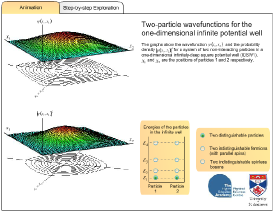
This flash animation shows you some examples of the above symmetrization postulates in case of two-particle wavefunctions for the one dimensional infinite potential well. Three different cases are demonstrated, namely two distinguishable particles, two fermions with parallel spin and two bosons with zero spin.
http://www.st-andrews.ac.uk/~qmanim/embed_item_3.php?anim_id=3
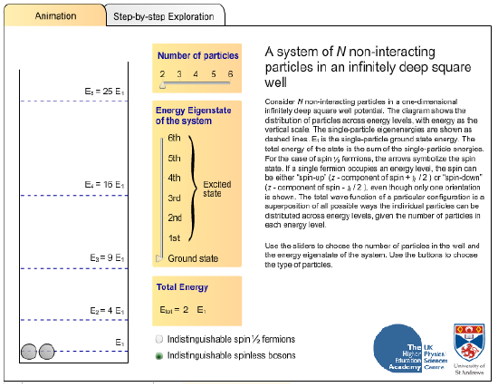
This flash animation guides you through the case of N non-interacting particles in an infinitely deep square well.
http://www.st-andrews.ac.uk/~qmanim/embed_item_3.php?anim_id=48
The one-electron approximation in atoms
The discussion given in the previous section can be extended to the approximate treatment of the electronic structure of atoms consisting of a nucleus with Z protons and a number N of identical electrons. The stationary states are the eigenfunctions of the following Hamiltonian:
\(H=\sum_{i=1}^{N} \frac{\mathbf{P}_{i}^{2}}{2 m_{e}}-\sum_{i=1}^{N} \frac{Z q_{0}^{2}}{4 \pi \epsilon_{0}} \frac{1}{\left|\mathbf{R}_{i}\right|}+\frac{q_{0}^{2}}{4 \pi \epsilon_{0}} \sum_{j<i} \sum_{i=1}^{N} \frac{1}{\left|\mathbf{R}_{i}-\mathbf{R}_{j}\right|}\) (6.26)
where we consider the nucleus fixed. In spite of the interaction described here by the third term, a surprisingly good approximation can be obtained by an iterated independent particle model, which we shall explain here. Let us note that the form of this Hamiltonian is a simplified one, there are in general spin dependent terms not contained in (6.26), but they can be neglected in the first approximation. Still, as we shall see, the spin of the particles shall influence the states indirectly through the antisymmetrization postulate given in the previous section.
It is impossible to determine the exact form of the spatial wave function \(\Psi\left(\mathbf{r}_{1}, \mathbf{r}_{2}, \ldots \mathbf{r}_{N}\right)\) by analytic or even by numerical methods, as it will be a function of \(3N\) variables in the spin independent case. Therefore we shall use the one-electron approximation, where we assume that if we consider a single electron separately from all the others, and the electron-electron interaction term (the last term in (6.26)) can be approximated by a potential energy of that single electron in the field of all the others. This potential energy function, which is to be written as \(V\left(\mathbf{R}_{i}\right)\) for the i-th electron, should depend only on the coordinate of that single electron. Mathematically this means that we make the following replacement
\(\sum_{i, j, i<j} \frac{1}{\left|\mathbf{R}_{i}-\mathbf{R}_{j}\right|} \longrightarrow \sum_{i} V\left(\mathbf{R}_{i}\right)\) (6.27)
So far we do not know the explicit form of \(V\left(\mathbf{R}_{i}\right)\), but the procedure we explain below will also yield us the expression of this potential energy. It may seem that we distinguish between the electrons by taking out one, but as we will see later, this will not be the case. We have then the following approximate Hamiltonian:
\(H^{i}=\sum_{i} h(i)\) (6.28)
where now
\(h(i)=\frac{\mathbf{P}_{i}^{2}}{2 m}-\frac{Z e_{0}^{2}}{R_{i}}+V\left(\mathbf{R}_{i}\right)\) (6.29)
is an effective one-electron operator that depends only on the coordinates of a single electron. Assume that we can find the solutions of the one-electron problem:
\(h(i) \varphi_{\alpha_{i}}\left(\mathbf{r}_{i}\right)=\varepsilon_{\alpha_{i}} \varphi_{\alpha_{i}}\left(\mathbf{r}_{i}\right)\) (6.30)
then the solution of
\(H^{i} \Psi\left(\mathbf{r}_{1}, \ldots, \mathbf{r}_{N}\right)=\sum_{i} h(i) \Psi\left(\mathbf{r}_{1}, \ldots, \mathbf{r}_{N}\right)=\mathcal{E} \Psi\left(\mathbf{r}_{1}, \ldots, \mathbf{r}_{N}\right)\) (6.31)
can be written as a product of so called one particle eigenstates \(\varphi_{\alpha_{i}}\left(\mathbf{r}_{i}\right)\):
\(\Psi_{H}\left(\mathbf{r}_{1}, \ldots, \mathbf{r}_{N}\right)=\prod_{\alpha_{i}} \varphi_{\alpha_{i}}\left(\mathbf{r}_{k}\right)=\varphi_{\alpha_{1}}\left(\mathbf{r}_{1}\right) \varphi_{\alpha_{2}}\left(\mathbf{r}_{2}\right) \ldots \varphi_{\alpha_{N}}\left(\mathbf{r}_{N}\right)\) (6.32)
\(\mathcal{E}=\sum_{i} \varepsilon_{\alpha_{i}}\) (6.33)
\(Ψ_{H}\) is a so called Hartree function, after D. Hartree, who first applied this approximation for multielectron atoms. The problem with \(Ψ_{H}\) is that it is not antisymmetric as prescribed by the antisymmetrization postulate, but we come soon to this point.
Show the validity of (6.31).
The method of Hartree intended to determine the ground state energy of the composite system. To this end he had chosen an initial set of N different wave functions, usually the well known eigenstates of lowest energy in a H-like atom with nuclear charge Z. The potential energy of the i-th single electron in the field of all others can be expressed by the spatial charge density of the other electrons:
\(\sum_{j e q i} \varrho\left(\mathbf{r}_{j}\right)=\sum_{j e q i}^{N} e_{0}^{2}\left|\varphi_{j}\left(\mathbf{r}_{j}\right)\right|^{2}\) (6.34)
according to
\(V\left(\mathbf{r}_{i}\right)=\sum_{j e q i}^{N} \int \frac{e_{0}^{2}\left|\varphi_{j}\left(\mathbf{r}_{j}\right)\right|^{2}}{\left|\mathbf{r}_{i}-\mathbf{r}_{j}\right|} d^{3} \mathbf{r}_{j}\) (6.35)
This is the Coulomb potential of the i-th electron created by the charge density of the other ones, and this is the effective one-electron potential. Now we can add this potential to the one-electron Hamiltonian, and we can solve the eigenvalue equation:
\(\left(-\frac{\hbar^{2}}{2 m} \Delta_{i}-\frac{Z e_{0}^{2}}{R_{i}}+V\left(\mathbf{r}_{i}\right)\right) \varphi_{i}\left(\mathbf{r}_{i}\right)=\varepsilon_{i} \varphi_{i}\left(\mathbf{r}_{i}\right)\) (6.36)
which will yield us new one-electron eigenfunctions \(φ_{i}(\mathbf{r}_{i})\) and energies \(ε_{i}\). From these functions we select those belonging to the lowest energy, and construct again a potential of the form (6.35), and then solve (6.36). In the k-th step of this iteration we solve thus
\(\left(-\frac{\hbar^{2}}{2 m} \Delta_{i}-\frac{Z e_{0}^{2}}{R_{i}}+\sum_{j e q i}^{N} \int \frac{e_{0}^{2}\left|\varphi_{j}^{(k-1)}\left(\mathbf{r}_{j}\right)\right|^{2}}{\left|\mathbf{r}_{i}-\mathbf{r}_{j}\right|} d^{3} \mathbf{r}_{j}\right) \varphi_{i}^{(k)}\left(\mathbf{r}_{i}\right)=\varepsilon_{i}^{(k)} \varphi_{i}^{(k)}\left(\mathbf{r}_{i}\right) .\) (6.37)
The procedure is to be repeated until the resulting potential differs from the one we started from by a given precision. The method is called therefore a self consistent field (SCF) method. In this way we can determine the charge density and the total energy of the ground state.
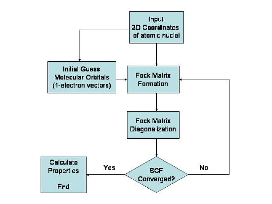
Figure 6.2: Simplified algorithmic flowchart illustrating the Hartree–Fock Method.
http://en.Wikipedia.org/wiki/Hartree-Fock_method
A serious problem with the SCF method of Hartree was, however, that in (6.32) the postulate of antisymmetry of the many-electron system was not taken into account. The Pauli principle can be satisfied only in its elementary form, which says that in the product (6.32) above, all the one-electron states must be different and orthogonal, or rather because of spin, the spatial part of a pair of electrons can be the same, as they can be multiplied by the two possible eigenstates of \(S_{z}\), as H is spin independent. This means that if we wish to determine the ground state of the N electron system we can choose those one-electron states in the product which belong to the lowest one-electron eigenvalues, where orbital and spin degeneracy must be taken into account, as well.
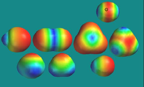
Figure 6.3: Electrostatic potential maps from Hartree-Fock calculations
http://science.csustan.edu/phillips/CHEM4610 Docs/CHEM4610_All Bonds Same.htm
In spite of satisfying the Pauli principle in its elementary form (each electron is in a different one-particle state), it does not obey the real requirement, which states that the wave function of identical fermions must be antisymmetric. Therefore the (6.32) product of functions must be antisymmetrized. In order to do so one has to construct the Slater determinant (6.23) out of the N functions we have chosen, and calculate the potential energy from this multiparticle wave function. This improved method was proposed by V. Fock and J. Slater independently and it is called the Harterre Fock (HF) method. We only quote the resulting equation here:
\(\left(-\frac{\hbar^{2}}{2 m} \Delta_{i}-\frac{Z e_{0}^{2}}{\left|\mathbf{r}_{i}\right|}+\sum_{j, j e q i}^{N} \int \frac{e_{0}^{2}\left|\varphi_{j}\left(\mathbf{r}_{j}\right)\right|^{2}}{\left|\mathbf{r}_{i}-\mathbf{r}_{j}\right|} d^{3} \mathbf{r}_{j}-\delta_{m_{i} m_{j}} \sum_{j, j e q i}^{N} \int e_{0}^{2} \frac{\varphi_{j}\left(\mathbf{r}_{j}\right) \varphi_{i}\left(\mathbf{r}_{j}\right)}{\left|\mathbf{r}_{i}-\mathbf{r}_{j}\right|} d^{3} \mathbf{r}_{j}\right) \varphi_{i}\left(\mathbf{r}_{i}\right)=\varepsilon_{i} \varphi_{i}\left(\mathbf{r}_{i}\right)\) (6.38)
which is called the Hartree-Fock equation. It differs from the Hartree equation by the last term on the left hand side. Due to the Kronecker delta \(\delta_{m_{i} m_{j}}\) it is present only for electrons with identical spin projections. Here again the left hand side contains the \(φ\)-s of \(k−1\)-th step, while on the right hand side we have already \(ε_{i}\) and \(φ_{i}(\mathbf{r}_{i}\) in the k-th step. It is to be repeated until self-consistency is achieved similarly to the case of the Hartree method, and it yields very good ground state energies and electronic densities for atoms.
We note that the HF method can be extended to calculate the electronic structure of molecules and solids. It is also worth to stress that there are many other approximate ways to find the electronic structure of atomic systems.
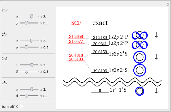
On this interactive animation we can investigate the lower excited states of a Helium atom. Besides the exact energy values results of SCF calculations is also shown. The SCF energy can be optimized by variation of some parameters which can be done by hand in the Demonstration. We can switch on and off the effect of exchange interaction to see how this interaction is responsible for the effect of the spin degrees of freedom.
http://demonstrations.wolfram.com/LowerExcitedStatesOfHeliumAtom/