6.3: Square Barrier

A slightly more involved example is the square potential barrier, an inverted square well, see Figure \(\PageIndex{1}\).

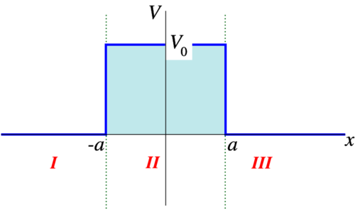
Figure \(\PageIndex{1}\): The square barrier.

We are interested in the case that the energy is below the barrier height, \(0< E< V_0\). If we once again assume an incoming beam of particles from the right, it is clear that the solutions in the three regions are

\[ \begin{align} ϕ_I ( x ) &= A_1 e^{i k x} + B_1 e ^{− i k x} \\[5pt] ϕ_{II} ( x ) &= A_2 \cosh ( κ x ) + B_2 \sinh ( κ x ) \\[5pt] ϕ_{III} ( x ) &= A_3 e^{ i k x}. \label{6.16} \end{align}\]

Here

\[k = \sqrt{\dfrac{2 m}{ℏ^2} E} \]

and

\[κ = \sqrt{\dfrac{2 m}{ℏ^2} ( V_0 − E )} . \label{6.17}\]

Matching \(ϕ_I\) and \(ϕ_{II} \) at \(x=− a\) and \(ϕ_{II}\) and \(ϕ_{III} \) at \(x= a\) gives (use \(\sinh (− x)=− \sinh x\) and \(\cosh (− x)= \cosh x\)).

\[ \begin{align} A_1 e^{−ika} + B_1 e^{ika} &= A_2 \cosh κ a − B_2 \sinh κ a \label{6.18} \\[5pt] i k ( A_1 e^{−ika} − B_1 e^{ika} ) &= κ ( − A_2 \sinh κ a + B_2 \cosh κ a ) \label{6.19} \\[5pt] A_3 e^{ika} &= A_2 \cosh κ a + B_2 \sinh κ a \label{6.20} \\[5pt] i k ( A_3 e^{ika} ) &= κ ( A_2 \sinh κ a + B_2 \cosh κ a ) \label{6.21} \end{align}\]

These are four equations with five unknowns. We can thus express for of the unknown quantities in one other. Let us choose that one to be \(A_1\), since that describes the intensity of the incoming beam. We are not interested in \(A_2\) and \(B_2\), which describe the wave function in the middle. We can combine the equation above so that they either have \(A_2\) or \(B_2\) on the right hand side, which allows us to eliminate these two variables, leading to two equations with the three interesting unknowns \(A_3\), \(B_1\) and \(A_1\). These can then be solved for \(A_3\) and \(B_1\) in terms of \(A_1\):

The way we proceed is to add Equations \ref{6.18} and \ref{6.20}, subtract Equations \ref{6.19} from \ref{6.21}, subtract \ref{6.20} from \ref{6.18}, and add \ref{6.19} and \ref{6.21}. We find

\[ \begin{align} A_1 e^{−ika} + B_1 e^{ika} + A_3 e^{ika} &= 2 A_2 \cosh κ a \label{6.22} \\[5pt] i k ( − A_1 e^{−ika} + B_1 e^{ika} + A_3 e^{ika} ) &= 2 κ A_2 \sinh κ a \label{6.23} \\[5pt] A_1 e^{−ika} + B_1 e^{ika} − A_3 e^{ika} &= − 2 B_2 \sinh κ a \label{6.24} \\[5pt] i k ( A_1 e^{−ika} − B_1 e^{ika} + A_3 e^{ika} ) &= 2 κ B_2 \cosh κ a \label{6.25} \end{align}\]

We now take the ratio of equations \ref{6.22} and \ref{6.23} and of \ref{6.24} and \ref{6.25}, and find (i.e., we take ratios of left- and right hand sides, and equate those)

\[ \begin{align} \dfrac{A_1 e^{−ika} + B_1 e^{ika} + A_3 e^{ika} }{i k ( − A_1 e^{−ika} + B_1 e^{ika} + A_3 e^{ika} )} &= \dfrac{1}{ κ \tanh κ a} \label{6.26} \\[5pt] \dfrac{ A_1 e^{−ika} + B_1 e^{ika} − A_3 e^{ika}}{ i k ( − A_1 e^{−ika} + B_1 e^{ika} + A_3 e^{ika} )} &= − \dfrac{\tanh κ a}{ κ} \label{6.27} \end{align}\]

These equations can be rewritten as (multiplying out the denominators, and collecting terms with \(A_1\), \(B_3\) and \(A_3\))

\[ \begin{align} A_1 e^{−ika} ( κ \tanh κ a + i k ) + B_1 e^{ika} ( κ \tanh κ a − i k ) + A_3 e^{ika} ( κ \tanh κ a − i k ) = 0 \label{6.28} \\[5pt] A_1 e^{−ika} ( κ − i k \tanh κ a ) + B_1 e^{ika} ( κ + i k \tanh κ a ) + A_3 e^{ika} ( − κ + i k \tanh κ a ) &= 0 \label{6.29} \end{align}\]

Now eliminate \(A_3\), add Equations \ref{6.28} and \ref{6.29} to find

\[\begin{array}{l} 
A_1 e^{-i k a}[ (\kappa-i k \tanh \kappa a)(\kappa \tanh \kappa a+i k)+ \\
(\kappa \tanh \kappa a-i k)(\kappa-i k \tanh \kappa a)] \\
+B_1 e^{i k a}[(\kappa-i k \tanh \kappa a)(\kappa \tanh \kappa a-i k)+ \\
(\kappa \tanh \kappa a-i k)(\kappa+i k \tanh \kappa a)]=0
\end{array}\]

Thus we find

\[B_1 = − A_1 e ^{− 2 i k a} \dfrac{ \tanh κ a ( k^2 + κ^2 ) }{( κ − i k \tanh κ a ) ( κ \tanh κ a − i k )} \label{6.31}\]

and we find, after using some of the angle-doubling formulas for hyperbolic functions, that the absolute value squared, i.e., the reflection coefficient, is

\[R = \dfrac{ \sinh^2 2 κ a \left( κ^2 + k^2 \right)^2}{ 4 κ^2 k^2 + \left( κ^2 − k^2 \right)^2 \sinh^2 2 κ a } \label{6.32}\]

In a similar way we can express \(A_3\) in terms of \(A_1\) (add Equations \ref{6.28} and Equation \ref{6.29}, or use

\[T= 1− R!\]

Alternative approach

The equation can be given in matrix form as

\[\begin{pmatrix} {e}^{−ika} & {e}^{ika}\\
ik{e}^{−ika}& -ik{e}^{ika}  \\
\end{pmatrix}\begin{pmatrix}
{A}_{1} \\{B}_{1} 
\end{pmatrix}
\begin{pmatrix}
\mathop{cosh}\nolimits κa & -\mathop{ sinh}\nolimits κa&  \\
-κ\mathop{ sinh} \nolimits κa & κ\mathop{ cosh} \nolimits κa \\
\end{pmatrix}\begin{pmatrix}
{A}_{2} \\{B}_{2} 
\end{pmatrix}\begin{pmatrix} 
{e}^{ika} & {e}^{-ika}\\
ik{e}^{−ika}& -ik{e}^{ika} \\
\end{pmatrix}\begin{pmatrix}
\mathop{cosh}\nolimits κa & \mathop{ sinh}\nolimits κa&  \\
κ\mathop{ sinh} \nolimits κa & κ\mathop{ cosh} \nolimits κa \\
\end{pmatrix}\begin{pmatrix}
{A}_{2} \\{B}_{2} 
\end{pmatrix} \]

Question: Can you invert the matrices and find the same answer as before?

Example \(\PageIndex{1}\): Hydrogen Atom Scattering

We now consider a particle of the mass of a hydrogen atom, \(m= 1.67 × 10^{−27} kg\), and use a barrier of height 4 meV and of width \(10^{−10} m\). The picture for reflection and transmission coefficients can seen in Figure \(\PageIndex{1; left}\). We have also evaluated \(R\) and \(T\) for energies larger than the height of the barrier (the evaluation is straightforward).

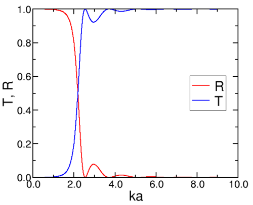
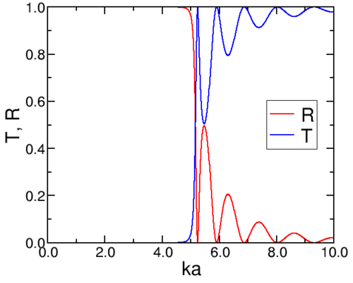
Figure \(\PageIndex{2}\): The reflection and transmission coefficients for a square barrier of height 4 meV (left) amd 50 meV (right) and width 1 0− 1 0 m.

If we heighten the barrier to 50 meV, we find a slightly different picture (Figure \(\PageIndex{1; right}\)).

Notice the oscillations (resonances) in the reflection. These are related to an integer number of oscillations fitting exactly in the width of the barrier, \(\sin^2κ a= 0\).