12.3.2: The Spin-Orbit Effect

In order to further explain the structure of the hydrogen atom, one needs to consider that the electron not only has orbital angular momentum \(\mathbf{L}\), but also intrinsic angular momentum \(\mathbf{S}\), called spin. There is an associated spin operator \(\mathbf{S}\), as well as operators \(S^2\) and \(S_z\), just as with \(\mathbf{L}\). Usually written in matrix form, these operators yield results analogous to \(L^2\) and \(L_z\) when acting on the wavefunction \(\Psi\),

\[\begin{aligned}
S^2 \Psi & =s(s+1) \hbar^2 \Psi \\
S_z \Psi & =m_s \hbar \Psi
\end{aligned}\]

where \(s\) and \(m_s\) are quantum numbers defining the magnitude of the spin angular momentum and its projection onto the \(z\)-axis, respectively. For an electron \(s=1 / 2\) always, and hence the electron can have \(m_s=+1 / 2,-1 / 2\).

Associated with this angular momentum is an intrinsic magnetic dipole moment

\[\mu_{\mathrm{S}}=-g_s \mu_b \frac{\mathbf{S}}{\hbar}\]

where

\[\mu_b \equiv \frac{e \hbar}{2 m c}\]

is a fundamental unit of magnetic moment called the Bohr magneton. The number \(g_s\) is called the spin gyromagnetic ratio of the electron, expected from Dirac theory to be exactly 2 but known experimentally to be \(g_s=\) 2.00232. This is to be compared to the magnetic dipole moment associated with the orbit of the electron,

\[\mu_{\mathrm{l}}=-g_l \mu_b \frac{\mathbf{L}}{\hbar}\]

where \(g_l=1\) is the orbital gyromagnetic ratio of the electron. That is, the electron creates essentially twice as much dipole moment per unit spin angular momentum as it does per unit orbital angular momentum. One expects these magnetic dipoles to interact, and this interaction constitutes the spin-orbit effect.

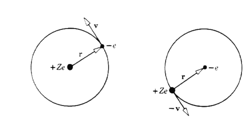
The interaction is most easily analyzed in the rest frame of the electron, as shown in figure 2. The electron sees the nucleus moving around it with speed \(v\) in a circular orbit of radius \(r\), producing a magnetic field

\[B=\frac{Z e v}{c r^2} .\]

Figure \(\PageIndex{1}\):On the left an electron moves around the nucleus in a Bohr orbit. On the right as seen by the electron the nucleus is in a circular orbit.

In terms of the electron orbital angular momentum \(L=m r v\), the field may be written

\[\mathbf{B}=\frac{Z e}{m c r^3} \mathbf{L}\]

The spin dipole of the electron has potential energy of orientation in this magnetic field given by

\[\Delta E_{s o}=-\mu_{\mathrm{S}} \cdot \mathbf{B} .\]

However, the electron is not in an inertial frame of reference. In transforming back into an inertial frame, a relativistic effect known as Thomas precession is introduced, resulting in a factor of \(1 / 2\) in the interaction energy. With this, the Hamiltonian of the spin-orbit interaction is written

\[\Delta H_{s o}=\frac{Z e^2}{2 m^2 c^2 r^3} \mathbf{L} \cdot \mathbf{S}\]

With this term added to the Hamiltonian, the operators \(L_z\) and \(S_z\) no longer commute with the Hamiltonian, and hence the projections of \(\mathbf{L}\) and \(\mathbf{S}\) onto the \(z\)-axis are not conserved quantities. However, one can define the total angular momentum operator

\[\mathbf{J}=\mathbf{L}+\mathbf{S}\]

It can be shown that the corresponding operators \(J^2\) and \(J_z\) do commute with this new Hamiltonian. Physically what happens is that the dipoles associated with the angular momentum vectors \(\mathbf{S}\) and \(\mathbf{L}\) exert equal and opposite torques on each other, and hence they couple together and precess uniformly around their sum \(\mathbf{J}\) in such a way that the projection of \(\mathbf{J}\) on \(z\)-axis remains fixed. The operators \(J^2\) and \(J_z\) acting on \(\Psi\) yield

\[\begin{aligned}
J^2 \Psi & =j(j+1) \hbar^2 \Psi \\
J_z \Psi & =m_j \hbar \Psi
\end{aligned}\]

where \(j\) has possible values

\[j=|l-s|,|l-s|+1, \ldots, l+s-1, l+s .\]

For a hydrogenic atom \(s=1 / 2\), and hence the only allowed values are \(j=l-1 / 2, l+1 / 2\), except for \(l=0\), where only \(j=1 / 2\) is possible. Figure 3 illustrates spin-orbit coupling for particular values of \(l, j\), and \(m_j\).

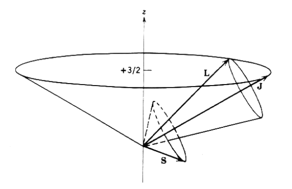
Figure \(\PageIndex{2}\): Spin-orbit coupling for a typical case of \(s=1 / 2, l=2, j=5 / 2\), \(m_j=3 / 2\), showing how \(\mathbf{L}\) and \(\mathbf{S}\) precess about \(\mathbf{J}\).

Since the coupling is weak and hence the interaction energy is small relative to the principle energy splittings, it is sufficient to calculate the energy correction by first-order perturbation theory using the previously found wavefunctions. The energy correction is then

\[\Delta E_{s o}=\left\langle\Delta H_{s o}\right\rangle=\int \Psi^* \Delta H_{s o} \Psi d^3 x .\]

The value of \(\mathbf{L} \cdot \mathbf{S}\) is easily found by calculating

\[J^2=\mathbf{J} \cdot \mathbf{J}=L^2+S^2+2 \mathbf{L} \cdot \mathbf{S}\]

and hence when acting on \(\Psi\),

\[\mathbf{L} \cdot \mathbf{S} \Psi=\frac{1}{2} \hbar^2[j(j+1)-l(l+1)-s(s+1)] \Psi .\]

One then needs to calulate the expectation of \(r^{-3}\), which is more complicated. The answer is

\[\Delta E_{s o}=\left(Z \alpha^4\right) m c^2 \frac{\left[j(j+1)-l(l+1)-\frac{3}{4}\right]}{4 n^3 l\left(l+\frac{1}{2}\right)(l+1)},\]

where the value \(s=1 / 2\) has been included.

Contributors and Attributions

• Randal Telfer (JWST Astronomical Optics Scientist, Space Telescope Science Institute)