
4.5: The Kronig-Penney Model
- Page ID
- 28764

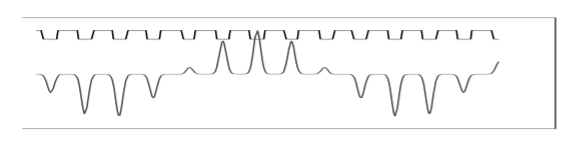
In 4.1 \(u(x)\) is still completely general. The Kronig-Penney model considers a periodically repeating square potential defined in one cell by \(V (x) = 0 (0 < x < b); V (x) = V_0 (b < x < l)\), then we can solve for \(u(x)\) in one cell. Like the finite square well, this is a tedious boundary condition problem where matching value and slope of the wavefunction at the potential edge gives a 4x4 matrix to diagonalise. The details are given in Wikipedia(!) and lead to an equation the LHS of which is drawn below:
\[\cos k_1b \cos k_2(l − b) − \frac{k^2_1 + k^2_2}{2k_1k_2} \sin k_1b \sin k_2(l − b) = \cos kl \nonumber\]
where \(k_1 = \sqrt{2mE}/\hbar\) and \(k_2 = \sqrt{2m(E − V_0)}/\hbar\), the appropriate free particle wavevectors, thus for \(E < V_0, k_2\) is imaginary. As the figure shows, multiple solutions are possible for all \(k\), giving certain “bands” of energy, but not others.
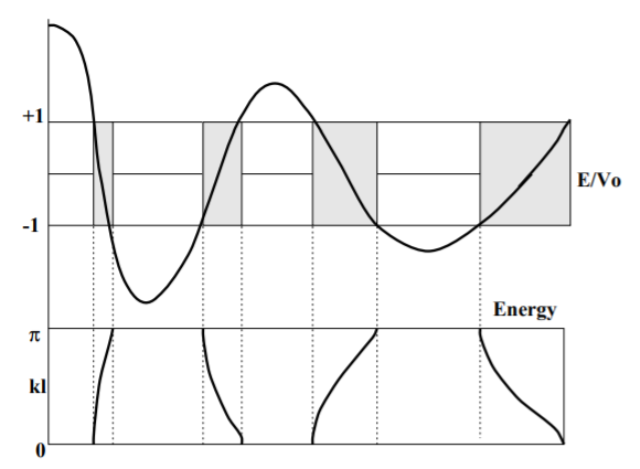
Figure \(\PageIndex{2}\): Graph of function arising from multiple square-well problem: Allowed energy solutions exist only where \(| \cos kl| \leq 1\).
The key point about this equation is that it cannot be solved for certain values of \(E\), around \(k_1b = m\pi \). A plot of the left hand side of the equation against \(E/V_0\) illustrates this, solutions for some value of \(k\) can be found only in the shaded regions of \(E\). Moreover each shaded region contains N allowed \(k = 2\pi n/Nl\) values. Thus if each atom contributes two electrons the lower ‘valence’ band will be filled (one of each spin in each state) and the upper ‘conduction’ band will be empty. To get an electron to move (change to a different \(k\)-state) requires a lot of energy, so this represents an insulator.
In the limit of \(V_0 = 0\), we get \(k = k_1 = k_2 = \sqrt{2mE}/\hbar\), the free electron result, while for very large \(V_0 >> E\) solutions are possible only for values of \(E\) which satisfy \(\sin (k_1 b) \approx 0\), i.e. the square well.
The wavefunction is a complex exponential of \(k_1x\) or \(k_2x\), depending on whether it is in a well or not. It is not and eigenfunction of the momentum operator. Thus although \(\hbar k\) looks like a momentum, it isn’t the eigenvalue of the momentum operator. It is called “crystal momentum” and along with the “effective mass” gives a pair of quantities with which we can apply Newtonian dynamics thinking to a crystal, ignoring the effects of the lattice.
In three dimensions, the topology of the bands becomes much more complicated: this is a topic for solid state physics.