Appendix

For the Instructor’s Use

An appendix filled with nonstop mathematical gore may seem like a strange tag onto a book intended to teach people about relativity using primarily pictures, containing only as many equations as are absolutely required. I nevertheless include it for instructors and those few readers who do not mind the math. I do so for three reasons. First, an arc-length claim is made in chapter 4 of this book that is given without visual proof, and readers might wish to know that such a proof exists. Second, one may want to determine time-dilation factors exactly for the accelerated portions of our trip to Alpha Centauri in chapter 3. Third, references that lay out relativistic relations that include acceleration without tensor analysis are almost nonexistent. An out-of-print book by Francis Sears and Robert Brehme* is the only one I have found.

To show that the arc length in figure 10 of chapter 4 is given by equation

\[\tau^{2}=1-\frac{2 A r}{c^{2}} t^{2}, \tag{A1}\]

(where A = GM/r²) and, ultimately, to get the Schwarzschild radius, one must first know the relations between position, coordinate time, and proper time in an accelerated system. One first correctly defines acceleration in terms of proper-time derivatives of the four-velocity,

\[X=\{c t, \vec{r}\}, \tag{A2a}\]

\[V=\frac{d X}{d \tau}=\left\{V_{t}, \vec{V}_{r}\right\}=c \gamma, \frac{d \vec{r}}{d \tau}, \tag{A2b}\]

where the superscript μ takes the values 0, 1, 2, and 3 referring to time and the three spatial coordinates. Notice that V is the derivative of position X with respect to the proper time and whose proper time derivative is the acceleration:

\[A=\frac{d V}{d \tau}=\left\{A_{t}, \vec{A}_{r}\right\}. \tag{A2c}\]

Note

*     F. W. Sears and R. W. Brehme, Introduction to the Theory of Relativity (Addison-Wesley, Reading, MA, 1968), p. 102 f

We also note that

\[\vec{v}=\frac{d \vec{r}}{d t} \tag{A2d}\]

and

\[\gamma=\frac{d t}{d \tau}. \tag{A2e}\]

Figure \(\PageIndex{1}\): Equations (A3a, b). Graphical depiction of relationships among invariant, spatial, and temporal components of various four-vectors. (CC BY-NC-ND; Jack C. Straton)

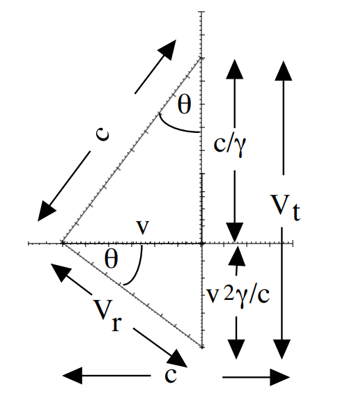
Now, from the Pythagorean theorem applied to the upper triangle in figure 1, or using the definition of the proper-time interval for a flat metric,

\[ \eta_{v}= \ \begin{array}{cccc} 1 & 0 & 0 & 0 \\ 0 & -1 & 0 & 0 \\ 0 & 0 & -1 & 0 \\ 0 & 0 & 0 & -1 \end{array} \nonumber\]

with the Einstein convention that repeated indices imply a sum over all possible values),

\[c^{2} d \tau^{2} \equiv d X d X=\eta_{v} d X d X^{v}=c^{2} d t^{2}-d r^{2}=\left(c^{2}-v^{2}\right) d t^{2} . \tag{A3a}\]

Then dividing by \( d \tau^{2}\),

\[ c^{2}=V_{t}^{2}-V_{r}^{2}\tag{A3b}\]

shows that the lower triangle in figure 1 is similar to the upper triangle. Finally, the \(\tau\) derivative of (A3b) gives

\[0=V_{t} A_{t}-V_{r} A_{r}=V A. \tag{A3c}\]

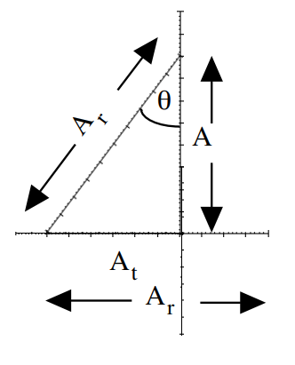
In the instantaneous rest frame of the uniformly accelerating rocket, \(V_{r}=0\) and \(V_{t} = c\) so that the angle θ in figure 1 goes to 0. In this case, (A3c) implies \(A_{t} = 0\). Then the spatial part of the acceleration four-vector in the instantaneous rest frame of the rocket (with θ = 0 in figure 2, the triangle equivalent to figure 1 for acceleration) gives the size of the invariant acceleration, \(A_{r}^{2}=A^{2}\), just as the temporal part of the momentum four-vector in the instantaneous rest frame of the rocket gives the invariant mass, \(E_{0}=m c^{2}\). A vector with the former properties is called space-like, and those with the latter (more conventional) properties are called time-like. This means that for θ > 0, figure 2 must have \(A_{r}\) on the hypotenuse.

Then this triangle is similar to the one for velocity only if the three-acceleration is parallel to the three-velocity. All the following assumes this restriction. We take both three-acceleration and three-velocity parallel to the x-direction for simplicity; then, from (A3c), \(A_{t} V_{t}=A_{x} V_{x}\). From figures 1 and 2,

\[\sin \theta=v / c=V_{x} / V_{t}=A_{t} / A_{x}, \tag{A4a}\]

\[\cos \theta=1 / \gamma=c / V_{t}=A / A_{x} \tag{A4b}\]

\[\tan \theta=\gamma v / c=V_{x} / c=A_{t} / A. \tag{A4c}\]

Figure \(\PageIndex{2}\): Equations (A4a–c). (CC BY-NC-ND; Jack C. Straton)

From \(\sec ^{2} \theta-\tan ^{2} \theta=1\), one may show that

\[A_{x}=A \sqrt{1+\left(V_{x} / c\right)^{2}} \tag{A5a}\]

or

\[\frac{d V_{x}}{\sqrt{1+\left(V_{x} / c\right)^{2}}}=A \ d \tau. \tag{A5b}\]

Since c and A are invariant constants, one may integrate* to obtain

\[V_{x}=c \sinh A \tau / c+\operatorname{arcsinh}\left(V_{x 0} / c\right), \tag{A6}\]

where we have set \( \tau_{o}=0\), and \(V_{x}\left(\tau=\tau_{0}=0\right)=V_{x 0} \). We integrate again† to obtain

\[X_{x}-X_{x 0}=\frac{c^{2}}{A}\left(\cosh \left[A \tau / c+\operatorname{arcsinh}\left(V_{x 0} / c\right)\right]-\sqrt{1+V_{x 0}^{2} / c^{2}}\right), \tag{A7}\]

where we have used \(\operatorname{arcsinh}(y)=\operatorname{arccosh}\left(\sqrt{1+y^{2}}\right) \). Using (A6) in (A5a),

\[A_{x}=A \cosh A \tau / c+\operatorname{arcsinh}\left(V_{x 0} / c\right). \tag{A8}\]

Dividing (A6) by (A8) and using (A4c) and (A4b), we have

\[v=c \tanh A \tau / c+\operatorname{arcsinh}\left(V_{x 0} / c\right). \tag{A9a}\]

Now using (A2e) and (A4b) in (A8) and integrating

\[d t=\gamma d \tau=\sec \Theta d \tau=\cosh A \tau / c+\operatorname{arcsinh}\left(V_{x 0} / c\right) d \tau \tag{A10}\]

yields

\[t=\frac{c}{A}\left(\sinh A \tau / c+\operatorname{arcsinh}\left(V_{x 0} / c\right)-V_{x 0} / c\right), \tag{A11}\]

where we have synchronized clocks at \( t_{0}=\tau_{o}=0\). Note that this is not \( \gamma \ \tau\): it is only for differentials (\( d t=\gamma d \tau\)) where this is true for accelerated systems. For extended durations, one must use (A11) and its inverse relation,

\[\tau=\frac{c}{A} \operatorname{arcsinh} \frac{A t+V_{x 0}}{c}-\frac{c}{A} \operatorname{arcsinh} \frac{V_{x 0}}{c}. \tag{A11a}\]

Also note that the limit is

\[t \rightarrow_{_{A \rightarrow 0}} \sqrt{1+\frac{V_{x 0}^{2}}{c^{2}}} \tau. \tag{A11b}\]

Inverting (A9a) gives

\[V_{x 0}=c \sinh -\frac{A \tau}{c}+\operatorname{arctanh} \frac{v}{c} \tag{A9b}\]

Note

*     I. S. Gradshteyn and I. M. Ryzhik, Table of Integrals, Series, and Products (Academic, New York, 1980), p. 99, No. 2.261(b).

†     I. S. Gradshteyn and I. M. Ryzhik, Table of Integrals, Series, and Products (Academic, New York, 1980), p. 155, No. 2.248.1.

and taking the same limit of the square of this, one recovers the special relativistic result,

\[t \rightarrow_{_{A \rightarrow 0}} \sqrt{1+\sinh ^{2}-\frac{A \tau}{c}+\operatorname{arctanh} \frac{v}{c}} \ \tau \rightarrow_{_{A \rightarrow 0}} \sqrt{1+\frac{v^{2}}{\left(c^{2}-v^{2}\right)}} \tau=\frac{1}{\sqrt{1-\frac{v^{2}}{c^{2}}}} \tau. \tag{A11c}\]

Using (A7) and (A11) in \( \cosh ^{2} \Phi-\sinh ^{2} \Phi=1\), one obtains

\[\frac{A\left(X_{x}-X_{x 0}\right)}{c^{2}}+\sqrt{1+\frac{V_{x 0}^{2}}{c^{2}}} ^{2}-\frac{A t}{c}+\frac{V_{x 0}}{c}^{2}=1, \tag{A12a}\]

which is the equation of a hyperbola, reducing to the equation for a parabola,

\[\left(X_{x}-X_{x 0}\right) \cong \frac{1}{2} A t^{2}+V_{x 0} t, \tag{A12b}\]

when \(A t<<c\) and \(V_{x 0}<<c\). * Relation (A12a) may also be derived by coordinate time integration, as shown in Sears and Brehme.†

Using (A7) in (A12a) gives

\[\sinh A \tau / c+\operatorname{arcsinh}\left(v_{x 0} / c\right)^{2}-\frac{A t}{c}+\frac{V_{x 0}}{c}^{2}=0. \tag{A12c}\]

Moving the second term to the right-hand side and taking the square root and then the derivative of both sides gives two useful differential relations:

\[d t=\cosh \frac{A \tau}{c}+\operatorname{arcsinh} \frac{V_{x 0}}{c} \ d \tau=\sqrt{1+\frac{A t}{c}+{\frac{V_{x 0}}{c}}^{2}} d \tau. \tag{A13}\]

The first equality can also be found by using (A4c), \(\gamma=V_{x 0} / v\), which is (A6) divided by (A9).

Also (A12a) gives a third form,

\[d t=\sqrt{1+\frac{V_{x 0}^{2}}{c^{2}}}+\frac{A\left(X_{x}-X_{x 0}\right)}{c^{2}} d \tau \tag{A14a}\]

and from (A9b) and (A14a)

\[\gamma=\sqrt{1+\sinh ^{2}-A \tau / c+\operatorname{arctanh}(\mathrm{v} / c)}+\frac{A\left(X_{x}-X_{x 0}\right)}{c^{2}}. \tag{A14b}\]

Note

*     The next higher terms in the series expansion of \(\sqrt{1+\frac{A t}{c}+\frac{V_{x 0}}{c}^{2}}-\sqrt{1+\frac{V_{x 0}^{2}}{c^{2}}}\) are \(-\frac{3}{4} \frac{V_{x 0}^{2}}{c^{2}}-\frac{1}{2} \frac{A t}{c} \frac{V_{x 0}}{c}-\frac{1}{8} \frac{A^{2} t^{2}}{c^{2}} \ A t^{2}-\frac{1}{4} \frac{V_{x 0}^{2}}{c^{2}} V_{x 0} t\).

†     F. W. Sears and R. W. Brehme, Introduction to the Theory of Relativity (Addison-Wesley, Reading, MA, 1968), p. 102 f

For small A, this simplifies to

\[\gamma \rightarrow_{_{A \rightarrow 0}} \frac{1}{A \rightarrow 0} \frac{1}{\sqrt{1-\frac{v^{2}}{c^{2}}}}+A\left(\frac{\left(X_{x}-X_{x 0}\right)}{c^{2}}-\frac{1}{\sqrt{1-\frac{v^{2}}{c^{2}}}} \frac{v \tau}{c^{2}}\right), \tag{A14c}\]

which reduces to the nonaccelerated value for A = 0.

Upon inverting (A13) and expanding the denominator in a series, one obtains

\[(d \tau)^{2}=1-\frac{2 A\left(X_{x}-X_{x 0}\right)}{c^{2}}-\frac{V_{x 0}^{2}}{c^{2}}+3 \frac{A\left(X_{x}-X_{x 0}\right)}{c^{2}}+\frac{1}{2} \frac{V_{x 0}^{2}}{c^{2}}+\frac{1}{4} \frac{V_{x 0}^{4}}{c^{4}}+\ldots(d t)^{2}, \tag{A15c}\]

of which (A1) is the first approximation if \( V_{x 0}=0\). Note that with A = 0, one regains the special-relativistic equation for time dilation at constant velocity \(V_{x 0}\) (which equals \(v_{0}\) in lowest order).

Finally, we note that the uniform acceleration of the rocket in the same direction as the change in position, as in figure 2a of chapter 4, feels like (is equivalent to) gravitational acceleration in the opposite direction to the change in position in figure 2b of chapter 4. So we replace

\[A_{\text {thrusters}} \ x -A_{\text {gravity}} \ r=-\frac{F_{g}}{m} \quad r=(-1)^{2} \frac{V(r)}{m}=\frac{G M}{r} \tag{A16}\]

to give* the Schwarzschild solution of chapter 4,

\[t^{2}=\frac{1}{1-\frac{1}{r} \times \frac{2 G M}{c^{2}}} \tau^{2}. \tag{A15b}\]

Alternatively, one can prove that the arc in figure 10 of chapter 4 really has length

\[c t=1+\frac{A \quad x}{c^{2}} c \tau. \tag{A17}\]

The relations derived above are necessary for this second proof. The arc-length is defined parametrically by

\[\begin{aligned} L &=c \int_{0}^{\tau} \sqrt{\frac{d x}{c d \tau}^{2}+\frac{d t}{d \tau}^{2}} d \tau \\ &=c \int_{0}^{\tau} \sqrt{1+2 \sinh ^{2} \frac{A \tau}{c}} d \tau. \end{aligned} \tag{A18}\]

where we have set \(V_{x 0}=0\).

Note

*     To obtain this from the above expression, we first redefine our distance coordinate as decreasing downward rather increasing downward as above, by changing the sign of all r’s. Next we note that mAr is just the gravitational potential energy −GmM/r.

As with elliptical integrals, one expands the radical in the small parameter \(A \tau / d\) and uses (A7) and (A11) to obtain

\[\begin{aligned} L &=c \int_{0}^{\tau} 1+\sinh ^{2} \frac{A \tau}{c}+\cdots d \tau \\ &=c \ \tau+\frac{c}{2 A} \sinh \frac{A \tau}{c} \cosh \frac{A \tau}{c}-\frac{1}{2} \tau+\cdots \\ &=\frac{c \tau}{2}+\frac{c^{2}}{2 A} \sinh \frac{A \tau}{c} \cosh \frac{A \tau}{c}-1+1+\cdots \\ &=\frac{c \tau}{2}+\frac{c t}{2} \frac{A\left(x-x_{0}\right)}{c^{2}}+1+\cdots, \end{aligned} \tag{A19a}\]

where we have set \( X_{x}=x\) and \( X_{x o}=x_{o}\) for a more conventional notation.

Finally, suppose the length of this arc is \(L=c t\) to first approximation, as labeled in figure 10 of chapter 4; then (A19a) becomes

\[c t \ 1-\frac{1}{2} \frac{A\left(x-x_{0}\right)}{c^{2}}+1+\cdots=\frac{c \tau}{2} \tag{A19b}\]

or

\[t \ 1-\frac{A\left(x-x_{0}\right)}{c^{2}}+\cdots=\tau, \tag{A19c}\]

giving (A14a) to first approximation. Thus, the assumption \(L=c t\) is a consistent one, showing that the gravitational red-shift factor is essentially just the stretched path-length for a beam of light in a gravitational field.

Finally, one may want a relation like (A12a) involving just position and velocity, which may be obtained by solving (A7) and (A9) using the relation \(\cosh ^{2} \Phi-\sinh ^{2} \Phi=1\),

\[v^{2}=\frac{V_{x 0}^{2}+2 A\left(x-x_{0}\right) \sqrt{1+\frac{V_{x 0}^{2}}{c^{2}}}+\frac{A\left(x-x_{0}\right)^{2}}{c}}{c^{2}+V_{x 0}^{2}+2 A\left(x-x_{0}\right) \sqrt{1+\frac{V_{x 0}^{2}}{c^{2}}+\frac{A\left(x-x_{0}\right)^{2}}{c}} }c^{2} \rightarrow_{_{V_{0}} \rightarrow 0} \frac{2 A\left(x-x_{0}\right)+\frac{A\left(x-x_{0}\right)^{2}}{c}}{c^{2}+2 A\left(x-x_{0}\right)+\frac{A\left(x-x_{0}\right)^{2}}{c}} c^{2}. \tag{A20a}\]

When A is small, this reduces to the nonrelativistic form for constant A:

\[\frac{1}{2}\left(v^{2}-v_{0}^{2}\right)=\int v d v=\int A d x=A\left(x-x_{0}\right). \tag{A20b}\]

It is generally more convenient to calculate v from A via the relation (A13):

\[d t=\sqrt{1+\frac{V_{x 0}^{2}}{c^{2}}}+\frac{A\left(x-x_{0}\right)}{c^{2}} d \tau \equiv \gamma d \tau \equiv \frac{1}{\sqrt{1-\frac{v^{2}}{c^{2}}}} d \tau, \tag{A21}\]

or

\[v \equiv c \sqrt{1-\frac{1}{\gamma^{2}}}=c \sqrt{1-\frac{1}{\sqrt{1+\frac{V_{x 0}^{2}}{c^{2}}+\frac{A\left(x-x_{0}\right)}{c^{2}}^{2}}}} \cong c \sqrt{1-\frac{1}{1+\frac{A\left(x-x_{0}\right)}{c^{2}}+\frac{1}{2} \frac{V_{x 0}^{2}}{c^{2}}^{2}}}. \tag{A22}\]

Then we can rewrite (A12a) as

\[\frac{A t}{c}+\frac{V_{x 0}}{c}=\gamma^{2}-1, \tag{A23a}\]

or

\[t=\frac{c}{A} \sqrt{\gamma^{2}-1}-\frac{V_{x 0}}{c}. \tag{A23b}\]

We can obtain the corresponding relation between distance and \(\gamma\) by solving (A21) for \(x-x_{0}\), which we also called \(r\) in chapter 3.

\[r \equiv\left(x-x_{0}\right)=\frac{c^{2}}{A} \gamma-\sqrt{1+\frac{V_{x 0}^{2}}{c^{2}}}. \tag{A24}\]

INITIAL ACCELERATION TOWARDS ALPHA CENTAURI

Let us use these to find how long it takes to boost a rocket to \(v=0.6 c \ (\gamma=1.25)\) at an acceleration of 1 g.* If the initial velocity with \(V_{x 0}=0\), we have from (A23b) t = 0.726536 yr. Likewise (A24) gives the distance traveled when this speed is reached, r = 0.242179 c yr.

Inverting (A9a),

\[\tau=\frac{c}{A}-\operatorname{arcsinh} \frac{V_{x 0}}{c}+\operatorname{arctanh} \frac{v}{c} \tag{A9c}\]

gives \( \tau=0.671462 \ \mathrm{yr}\), as does inverting (A11a),

\[\tau=\frac{c}{A} \operatorname{arcsinh} \frac{A t+V_{x 0}}{c}-\operatorname{arcsinh} \frac{V_{x 0}}{c}. \tag{A11d}\]

We can use this to confirm the caution after equation (A11) that for extended periods of acceleration, the ratio \(t / \tau=1.08\) is indeed not \(\gamma=1.25\) even though we still have \(v=c \sqrt{1-\frac{1}{\gamma^{2}}}\) if \(\gamma\) is defined as in equation (A22).

Note

*     A 1 g acceleration can be written in the useful form A/c = 1/(0.968715 yr).

CONTINUOUS ACCELERATION TO CYGNUS X-1

Suppose we want to travel out to the black hole Cygnus X-1, 7,733 light-years away* in the shortest reasonable time. The rocket would accelerate at 1 g for half the trip, flip over and decelerate at 1 g for the remainder of the trip. At this acceleration, the rocket will reach the halfway point with a time-dilation factor given by (A21) of

\[\gamma=\sqrt{1+\frac{V_{x 0}^{2}}{c^{2}}}+\frac{A}{c} \frac{\left(x-x_{0}\right)}{c}=1+\frac{1}{0.98715 \ y r} \frac{(3866.5 \ c \ y r-0)}{c}, \nonumber\]

or \(\gamma=3,992.37\). Equation (A22) gives the rocket’s velocity as it just reaches the halfway point, \(r=3,866.5 \ c \ y r\), as \(v=c \sqrt{1-\frac{1}{\gamma^{2}}}=0.99999997 \ c\). Equation (A23b), with \(V_{x 0}=0\), gives the time for the half trip at \(t=\frac{c}{A} \sqrt{\gamma^{2}-1}=3,867.47 \ y r\), where we use the Julian year of 365.25 days as preferred by the IAU.^† Both equations (A9c) and (A11d) give \(\tau=8.70418 \ \mathrm{yr}\).

In chapter 4, we said that under large acceleration, “figure 1c will stretch out as in figure 1d, so much so that the curved light path will differ little from the straight hypotenuse. Both high constant speeds and large accelerations (to high speeds) give enormous time dilation.” We can now quantify these two claims in the present case of 1 g acceleration. The hypotenuse of the triangle under the hyperbolic curve shown in figure 1d, whose legs are r and \(c \tau\) (as calculated above using the correct formula for acceleration [A9c] or [A11d]), is \(c t^{\prime}=3,866.51 \ c \ y r\), just under 1 light-year shorter than the hyperbola, whose length is c t = 3,867.47 yr, a 0.02 % difference.

The intermediate constant velocity that would give such a triangle is \(r / t=0.999997 \ c\), indeed a high constant speed, differing in the sixth decimal place from the rocket’s velocity as it just reaches the halfway point. It would give a very big time dilation factor when calculated in the special-relativistic manner: \(t^{\prime} / \tau=444\). But the frame-shifting a rocket undergoes when accelerated at 1 g leads to a time dilation factor nearly ten times larger, \(\gamma=3,992.37\) when calculated using the correct (and consistent) formula for acceleration (A21). We see that our intuitive connection between the two cases falls well short of the reality, a divergence that will only grow as we go to even larger accelerations (to much higher speeds).

Note

*     The 2018 Gaia DR2 catalogue shows a parallax of 0.4218 mas, which gives d = 1/0.0004218 = 2371 pc = 7733 c yr. “DR2 2059383668236814720,” Centre de Données astronomiques de Strasbourg, last modified May 26, 2020, http://simbad.u-strasbg.fr/simbad/si...ments#lab_meas. Other names one can use for the search include HD 226868 and 1956+350.

†     G. A. Wilkinson, IAU Style Manual Comm. 5, in IAU Transactions XXB (unpublished pamphlet), 1987, p. S23, https://www.iau.org/static/publicati...manual1989.pdf (accessed June 26, 2020); https://www.iau.org/publications/pro...s_rules/units/ (accessed June 26, 2020).