
1.5: Cosmology
- Page ID
- 28818

THE BIG BANG
One of the more interesting applications of the general theory of relativity is in cosmology. In 1927, Georges Lemaître published a paper attempting to reconcile the massless cosmological solution of general relativity by Willem de Sitter, which explained “the observed receding velocities of extra-galactic nebulæ,” and Einstein’s own solution containing mass but including a cosmological constant to make for a static universe. Lemaître’s solution did reconcile them and provided a value for the relation between the recessional velocities of the galaxies and their distances, 625 km per second for every 1 million parsecs the galaxies are away from us.* That is, nearby galaxies are sluggishly moving away from us, while the farthest galaxies are sprinting.
Two years later, Edwin Hubble (after whom the space telescope is named) used his own improved observations to derive a more accurate constant. Hubble’s work became widely known, while Lemaître’s prior explication of what became known as the Hubble law did not, in part because Lemaître left his value out of the 1931 English translation, since he felt that better values had subsequently been offered.† It was only in 2018 that the International Astronomical Union (IAU) recommended that the law henceforth be known as the Hubble–Lemaître law.
This law suggests that we may be in the middle of some cosmic explosion of galaxies. In 1936, Robertson and Walker found a solution to Einstein’s equations in which the universe could have expanded outward from an infinitely dense state.‡ In 1948, Ralph Alpher and Robert Herman showed that as this expanding universe cooled from its inconceivably high initial temperature to a mere billion degrees in the first 200 seconds or so, about 1/4 of the hydrogen nuclei would have been transformed into helium nuclei. This is exactly the proportion of helium to hydrogen that is observed in the universe. They also estimated that this cooling would have continued for the subsequent 15–20 billion years until today, when one should see the ghost of this explosion as microwave radiation with a temperature of about 5 degrees above absolute zero, or 5 Kelvins (K; room temperature is 300 K).§ In 1965, Arno Penzias and Robert Wilson observed this background microwave radiation at a temperature of 3 K,¶ so the Big Bang appears to be confirmed.
Note
* G. Lemaître, Annales de la Société Scientifique de Bruxelles A47, 49–59 (1927).
† The relevant passage in the original is “Utilisant les 42 nébuleuses figurant dans les listes de Hubble et de Strômberg (1 ), et tenant compte de la vitesse propre du soleil (300 Km. dans la direction α = 315°, δ = 62°), on trouve une distance 0,95 millions de parsecs et une vitesse radiale de 600 Km./sec, soit 625 Km./sec à 10° parsecs (2).” Abbé G. Lemaître, MNRAS 91, 483–90 (1931).
‡ H. P. Robertson and A. G. Walker, Proc. London Math. Soc. 42, 90 (1936).
§ R. A. Alpher and R. C. Herman, Nature 162, 774 (1948); Phys. Rev. 75, 1089 (1949).
¶ A. A. Penzias and R. W. Wilson, Astrophys. J. 142, 419 (1965).
You actually know enough now to see how a Big Bang would work. Throughout this book, we have been using a pattern in which we relate proper time to coordinate time and coordinate distance. In chapter 1’s discussion of special relativity, we saw that the Pythagorean theorem applied to the light path in a ship moving at speed v relative to the Earth gave the full spacetime relation for proper time,‡
\[\tau^{2}=t^{2}-\frac{1}{c^{2}} r^{2} \tag{1}\]
For an accelerating rocket ship, or the equivalent observer in a gravitational field, the equivalent relation is
\[\tau^{2}=1-\frac{2 G M}{r c^{2}} t^{2}-\frac{1}{c^{2} \ \ 1-\frac{2 G M}{r c^{2}}} r^{2}+\text { angular terms } \tag{2}\]
where a full accounting would include angular spatial terms§ as well as the radial one we concentrated on in chapter 4, but those play no part in the discussion that follows.
Comparing this with time dilation in special relativity, you may see a symbolic pattern emerging in the shape of the equations, even had you not gone through the details of the idea in pictures. For the Robertson-Walker relation that describes the expansion of the universe, we might expect to see some quantity that changes with coordinate space and time multiplying the t2 term minus another quantity multiplying the r2 term. It turns out that the correct relation is
\[\tau^{2}=t^{2}-R^{2} \frac{1}{\left(1-k r^{2}\right) c^{2}} r^{2}+\text { angular terms } \tag{3} \]
R is a quantity that changes with time (often expressed by the notation R(t)) and so shows us how the intergalactic distances involving r and angles change with time. This cosmic scale factor is most easily thought of as the radius of a four-dimensional cosmic balloon, a hypersphere, that has as its outer surface our three-dimensional space. Now we do not have the ability to draw a four-dimensional balloon, but we can get an idea of how this would work if we discard one of our three spatial dimensions, as usual, and look at a spacetime of two spatial dimensions wrapping around the surface of a balloon, with the time dimension along its radius.
Note
‡ We can set v t = r in \(\tau^{2}=t^{2}-\frac{1}{c^{2}} v^{2} t^{2}-t^{2}-\frac{1}{c^{2}} r^{2}\).
§ See, for instance, Ronald Adler, Maurice Bazin, and Menachem Schriffer, Introduction to General Relativity (McGrawHill, New York, 1975), p. 225.
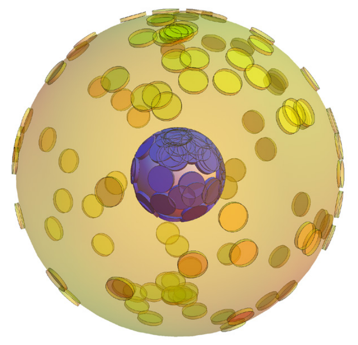
Figure \(\PageIndex{1}\) is a representation of the universe in two spatial dimensions lying on the surface of a sphere whose radius grows larger with time. As the universe doubles in size, the galaxies—originally arbitrarily colored yellow at the initial time and red at the later time to distinguish them—have moved outward on the expanding sphere and have simultaneously been dragged apart by the expanding universe without the galaxies changing size. A yellow galaxy sits at about the three o’clock position on the edge of our view of the universe at its initial size, with a second galaxy just above it, and a third just above that. As the universe doubles in size, the corresponding, now-red, galaxies move twice as far apart.
A blue arrow adjacent to the yellow galaxies shows the center-to-center distance between the first and second yellow galaxies. Its length is the disk diameter, and we will use that as the unit of measure. A second blue arrow combined with the first shows that the centerto-center distance between the first and third yellow galaxies is two disk diameters.
After the universe has doubled in size, the center-to-center distance between the first and second now-red galaxies has doubled to two disk diameters. Put another way, its position relative to the first has gotten one disk diameter larger. This additional distance is shown by the green arrow above the lowest blue arrow adjacent to the red galaxies.
Notice that after the universe has doubled in size, the center-to-center distance between the first and third now-red galaxies has also doubled, in this case to four disk diameters. Put another way, its position relative to the first has gotten two disk diameters larger. This additional distance is shown by the two green arrows in addition to the two blue arrows.
Since we define a velocity as the change in distance divided by the time interval, the recessional velocity of the third galaxy from the first is therefore twice the recessional velocity of the second galaxy from the first, since we are dividing by the same time interval in both measurements. This is precisely the Hubble–Lemaître law.
The scale of the universe is expanding and drags the galaxies apart with it. Note that in such a scheme, every galaxy would see every other galaxy receding, and we thus avoid the idea that we are at the center of the universe. To see this, just reverse the arrows in Figure \(\PageIndex{1}\) to see that galaxy 1 is moving away from galaxy 3 as much as the reverse is true. So creatures living in galaxy 3 will also come up with the Hubble–Lemaître law—though of course named for one of their own.
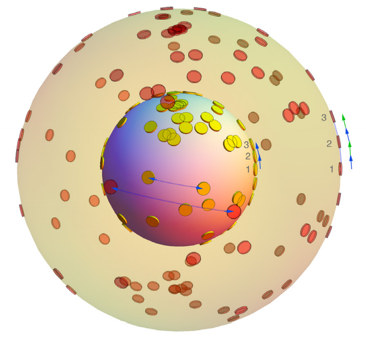
Figure \(\PageIndex{1}\): A representation of the universe in two spatial dimensions as lying on the surface of a sphere whose radius grows larger with time. The yellow disks lying on the inner sphere represent galaxies whose diameters are extremely exaggerated in size relative to the circumference of the universe. As the universe doubles in size, the galaxies—now red to distinguish the two times—have moved outward on the outer surface and have been dragged apart by the expanding universe without the galaxies changing size. A yellow galaxy sits at about the three o’clock position on the edge of our view of the universe at its initial size, with a second galaxy just above it and a third just above that. As the universe doubles in size, the corresponding, now-red, galaxies move twice as far apart.
The blue arrows adjacent to the yellow galaxies may be used to count the center-to-center distance between the first, second, and third galaxies as the universe expands. The green arrows add to the blues ones and represent the change in distance, which we divide by the time interval to get the recessional velocities. The distance from the first to the third galaxy has grown by two green arrows, while the distance from the first to the second galaxy has grown by only one green arrow, so the recessional velocity of the third from the first is twice that of the second galaxy from the first. This is the meaning of the Hubble–Lemaître law. (CC BY-NC-ND; Jack C. Straton)
Figure \(\PageIndex{1}\) also shows that the sizes of the galaxies (disks) do not change as their distance apart grows, nor do our local rulers grow with time, nor our noses. This is true for two reasons. First of all, the expansion equations showing an expanding universe are based on the idea that the universe is homogeneous, which holds true only on a large scale. The universe is decidedly lumpy on the scale of galaxies, solar systems, rulers, and atoms. Second, even if we could prove that a lumpy cosmology would expand, the gravitational attraction of nearby stars would overwhelm any cosmic tendency for galaxies to expand. And our bodies are held together by electrical forces that are (locally) enormously stronger than gravitational ones. (Otherwise we would fall through the chairs we sit on.) However, in an accelerating expansion that we will discuss in a minute, both local gravity and even electrical attraction may eventually be overwhelmed.
Finally, the question always comes up, “What is the universe expanding into?” If we were living in the universe of Figure \(\PageIndex{1}\) in the yellow-galaxy era, there would be no outer surface with red galaxies sitting on it. We could take a photograph inward from our surface into the past, but to photograph outward would be to photograph the future, and that is something no one I know is skilled at. From this perspective, one might say, “There is nothing there for the universe to expand into, and by ‘nothing’ I don’t mean emptiness of some sort but nonexistence. The universe must make the universe it is expanding into!”
Remember that Figure \(\PageIndex{1}\) is a representation of the universe in two spatial dimensions lying on the surface of a sphere whose radius grows larger with time. Put another way, in this picture, time is synonymous with the radius of the sphere. As time gets big, the sphere’s radius gets big in exact proportion. So for a spherical universe, one might answer, “The universe is expanding into the future!”
If you are satisfied with the Hubble–Lemaître law as given above, you may skip the following section that actually proves the Hubble–Lemaître law using some fairly complicated visual relationships.
THE HUBBLE–LEMAÎTRE LAW
We can show how the Hubble–Lemaître law works in more detail using Figure \(\PageIndex{2}\), a cross section of the four-dimensional hypersphere of Figure \(\PageIndex{1}\), but now with the added complication of a universe that is slowing its expansion velocity as time progresses. This slowing is what one would expect as the mass of all the rest of the universe tugs backward on the speed of every individual galaxy.
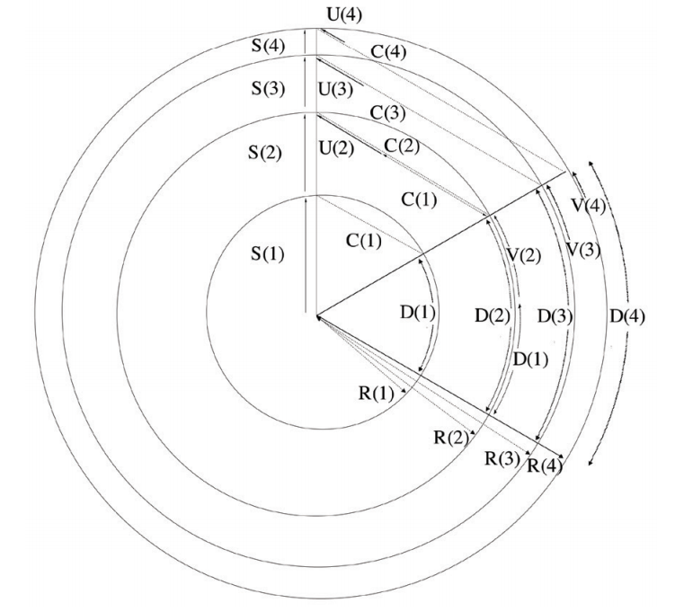
Figure \(\PageIndex{2}\): Consider the cross section of a spherical, expanding universe whose expansion rate S is slowing with time. R is the cosmic scale factor and, in the spherical case, is equal to the radius of the sphere. D is the arc of a circle, giving the distance between two galaxies exactly 60° around the curve from each other. V is the recessional speed of one galaxy, at the 2 o’clock position, from the one at the 4 o’clock position around the circumference of the circle—the change in D with time. The distance D at time 1, D(1), has been duplicated and shifted outward and placed next to D(2). The additional distance that must be added to D(1) to make the full distance D(2) is one time unit multiplying V(2), the recessional velocity at time 2. As the universal expansion slows, the recessional velocities also get smaller at times 3 and 4.
It may be easier to see distances and their changes over time by looking at equilateral triangles rather than arcs of circles. Thus, we also show C, the chord of the arc D, adjacent to a different 60° pie slice for visual clarity. The corresponding change in chord length from C(1) to C(2) with time is one time unit multiplying the velocity U(2). Since the chords are proportional to the arcs, U(2) is therefore proportional to the actual recessional velocity V(2). (CC BY-NC-ND; Jack C. Straton)
For a galaxy at the 12 o’clock position, exactly 60° around the curve from where we are at the 2 o’clock position in Figure \(\PageIndex{2}\), the distance across the chord between the galaxies equals the radius of the universe, because they are two sides of an equilateral triangle. This is true for any time: \(C(t)=R(t)\). Then the velocity U, the change in C with time, is precisely the expansion speed of the universe (the change in R with time) in this 60° case, or \(U(t) = S(t)\). Let us define a Hubble constant (as it is called, though it changes with time) at the present time \(H(4)=H_{0}\) as the ratio of the present expansion speed divided by the present radius: \(H_{0} \equiv S(4) / R(4)=U(4) / C(4)\) for galaxies in this 60° case. The Hubble–Lemaître law is simply a rewriting of this relation, giving the recessional velocity as proportional to the distance, \(U(4)=H_{0} C(4)\), with H0 as the constant of proportionality.
The actual distances between, and velocities of, galaxies are along the circumference, not across the chord, but those are in proportion. We check this by using the arc lengths in Figure \(\PageIndex{2}\), laid out in a different 60° pie slice for visual clarity, using a galaxy at the 4 o’clock position exactly 60° around the curve from where we are at the 2 o’clock position. It turns out that an arc of a circle has length R\(\theta\), where the angle \(\theta\) is expressed in fractions of the circumference (2 \(\pi\) R) of a circle that has radius 1, and thus as fractions of 2\(\pi\). For our case, 60° is 1/6 of the circumference so \(\theta\) = \(\pi\)/3 = 1.05 to three decimal places. (As you eyeball Figure \(\PageIndex{2}\), you might agree that the arcs could be about 5% larger than the chords.) As noted in the previous paragraph, the length of the chord across this 60° arc is precisely R, because they are two sides of an equilateral triangle. The adjacent arc has length 1.05 R for our 60° case. So if we just multiply all chord lengths C and their corresponding velocities U by 105%, we get the actual galactic distances D and recessional velocities V. But since we are taking ratios, this factor of 1.05 cancels out for any time: \(V / D=(1.05 \ U) /(1.05 \ C)=1.05 / 1.05 \ U / C =1 \ U / C=S / R=H_{0}\) , or \(V=H_{0} D\).
The arcs have the advantage of being able to be divided into smaller pie wedges whose arc lengths are easily seen. Suppose we imagine a galaxy at the 3 o’clock position at time 4, only 30° around the curve from where we are at the 2 o’clock position. Its distance from us will be half of D(4). We can also split the corresponding recessional velocity V(4) up into two parts, half associated with the 4 o’clock galaxy’s motion away from the 3 o’clock galaxy, and half associated with the 3 o’clock galaxy’s motion away from us at the 2 o’clock position. Looking at each half, we see that \((D(4) / 2) /(V(4) / 2)=D(4) / V(4)=H_{0}\) yet again, so the Hubble–Lemaître law holds for galaxies at any distance from us.
We are used to seeing the relationship between velocity and distance written as \(D = V T\), so we see that the Hubble constant is the inverse of some time, \(H_{0} = 1/T\). T turns out to be an estimate of the age of the universe, good to about 60% accuracy.
BUT IS THE UNIVERSE A FOUR-DIMENSIONAL SPHERE?
The constant \(k\) in Equation (3) tells us about the shape of the universe. The balloon scenario is accurate only if \(k = +1\). Since this universe has no edge, if you waited long enough, you would eventually see light from the back of your head that had traveled all the way around the four-dimensional hypersphere to your eyes.
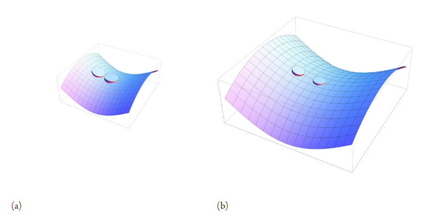
If \(k = −1\), then space is infinite and boundless, part of which is the saddle shape shown in Figure \(\PageIndex{3}\).
For \(k = 0\), Equation (3) looks very much like Equation (1), with only the addition of the scale factor R that allows the universe to grow with time. Thus, in this case, as for special relativity, space is flat. For this to be the case, the density of the universe must be at a critical value given by the Hubble constant and Newton’s gravitational constant G as \(\rho_{c}=\frac{3 H_{0}^{2}}{8 \pi G}\).
For a spacetime like that given by the Robertson-Walker metric Equation (3) (and more generally, Friedmann–Lemaître spacetimes), something called the Friedmann equation gives the expansion velocity of the universe. In the matter-dominated era, it can be shown that the square of the ratio of the expansion velocity of the universe S to the speed of light is
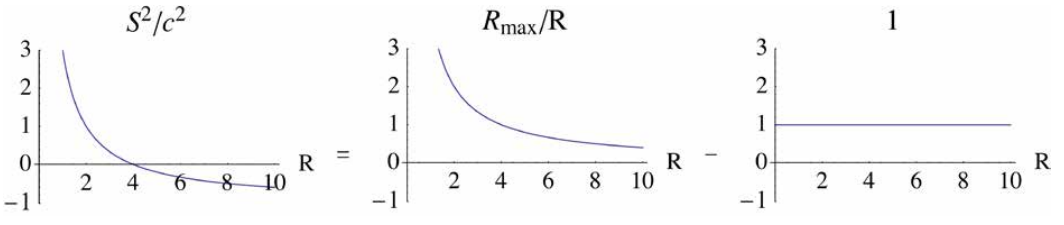
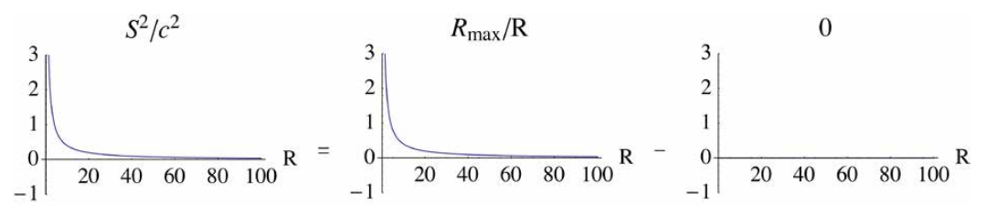
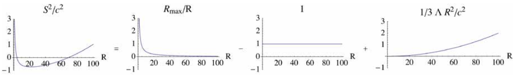
\[S^{2} / c^{2}=R_{\max } / R-k. \tag{4a}\]
When we look at the Hubble expansion in a k = 1 universe, we see that the expansion velocity S goes to zero at
\[R=R_{\max }, \tag{5}\]
since one then would have \(S^{2} / c^{2}=1-1=0\). (Here \(R_{\max }\) is given* in terms of the current radius R0 and current density \(\rho_{o}\) of the universe as \(8 \pi G / 3 \rho_{o} R_{0}^{3} / c^{2}\), in which we must have \(\rho_{0}>\rho_{c}\) for \(k\) to be 1.) But the mass is still exerting a force on the universe when it has stopped expanding, so we have a big crunch coming.
For those of you not familiar with looking for patterns in equations with your mind’s eye, let us cast Equation (4a) into a form for more conventional vision. If we arbitrarily set \(R_{\max }=4\), then as R increases from 0 to 10, the ratio \(R_{\max } / R\) drops from a high value to 0.4 at R = 10. This is the second picture in Equation (4b). Next we have \(k\) = 1 for all R from 0 to 10, the third picture in Equation (4b). If we subtract off the third picture from the second picture, we get the first picture, \(S^{2} / c^{2}\), with the dropping curve shifted downward by 1 unit at every point and becoming 0 at \(R=R_{\max }=4 \):
(4b)
(CC BY-NC-ND; Jack C. Straton)
When we look at the Hubble expansion in a k = 0 universe, the only value of R that will make \(S^{2} / c^{2}=0\) in Equation (4a) is R = ∞, as one can see by trying a series of larger values of R for Rmax arbitrarily set to 4 units: 4/100 = 0.04, 4/1000 = 0.004, 4/10000 = 0.0004, and so forth.
This is also seen in the k = 0 universe pictured in Equation (4c). We have extended R 10 times farther than in Equation (4b), and even at R = 100, the curve seems already at 0. In this case, the third picture has k = 0 for all values of R, so the subtraction of 0 does nothing, and the first picture for S2/c2 just duplicates the second one, going to 0 as R → ∞:
(4c)
(CC BY-NC-ND; Jack C. Straton)
When we look at the Hubble expansion in a \(k = −1\) universe, subtracting a negative is equivalent to adding a positive (−(−1) = +1) and there is no value of R that will make S2/c2 = 0, since we will always have the 1 left over, however small Rmax/R becomes. In Equation (4d), the first picture has the Rmax/R of the second picture shifted upward to approach 1. This universe will go on expanding forever.
Note
* Tai L. Chow, Gravity, Black Holes, and the Very Early Universe an Introduction to General Relativity and Cosmology (Springer, New York, 2008), p. 142, eq. (8.42).
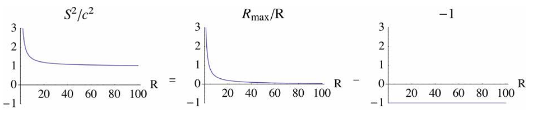
(4d)
(CC BY-NC-ND; Jack C. Straton)
So now we must somehow choose which shape (k = 1, 0, or −1) fits our universe.
THE BANG
One naturally wonders why the universe is expanding at all. Indeed, we can run the movie backward in our imagination, seeing the galaxies coming closer together as we move backward in time, as in Figure \(\PageIndex{4}\). Their initial, yellow, configuration becomes denser as time goes backward, with galaxies overlapping as the universe shrinks to a third of that size, shown in blue. As time runs down to zero, the spacetime containing the matter that makes up the galaxies turns into an infinitely dense dot that would also be extremely hot due to the friction of the jostled particles as they are forced into a smaller and smaller volume.
Such a visualization led to the idea of the Big Bang—that an initial singularity of infinitely dense, hot matter somehow exploded outward and is continuing to fly outward to this day, cooling as it expands.
AN OPEN AND SHUT CASE
What would cause the shape of the universe to curve in on itself, as in Figure \(\PageIndex{1}\), or flop open, as in Figure \(\PageIndex{3}\), or to take on perfect flatness? One may profitably ask a parallel question, “What causes an umbrella to close?” Well, you cause it to close by pulling down on the ring surrounding the handle, which in turn tugs inward on the spokes that attach to the clothcovered ribs. There are a few umbrellas that I have had a pretty hard time closing because I could not exert sufficient force to counter the outward pressure of the spring.
Suppose you had a universe that had enough mass that the inward gravitational force (in Newtonian language) could slow the outward expansion, bring it to a halt, and then cause it to recollapse in a Big Crunch. This is the k = +1 case. Suppose you had a universe that had insufficient mass to counter the outward momentum of the explosion of galaxies that is the Big Bang. That universe would not curl in on itself into a sphere but stay open like a floppy umbrella. This is the k = −1 case. There would, then, be some critical density of matter, \(\rho_{c}=\frac{3 H_{0}^{2}}{8 \pi G}\), just sufficient to halt the outward expansion at infinite time. This is the k = 0 case. *
We saw in the last section that running the closed, spherical-universe, k = +1 case backward in time led to an infinitely dense pinpoint singularity from which the Big Bang expanded outward. What about the other two, the open- and critical-universe cases where our universe is presently a saddle shape of infinite extent or flat and infinite? As one looks at Figure \(\PageIndex{5}\), one sees in either case a universe at present at the top becoming denser and denser as one proceeds downward, back in time.
No matter how far to the left the galaxies move, as we go backward in time to create increasing density, there will always be an infinite number of additional galaxies to the right moving into our frame of view. Thus, we can have an infinitely dense universe that is infinitely large just before the Big Bang occurred.
So in the k = 0 or k = −1 cases, the universe would not all be stuffed within a single point, as it would be if k = +1, but the entire infinite universe is nevertheless infinitely dense. In these cases, the Big Bang did not expand from a single point but from everywhere in the universe, and the scale of the universe, R, has been increasing ever since.
Note
* Before rescaling r to give k unit magnitude, k is given by \( \frac{k}{R_{0}^{2}}=\frac{8 \pi G}{3 c^{2}}\left(\rho_{0}-\rho_{c}\right)\) where \( \rho_{c}=\frac{3 H_{0}^{2}}{8 \pi G}\) is the critical density, \(\rho_{0}\) is the present density of the universe, R0 is its present size, H0 is the Hubble constant, and G is the universal gravitational constant.
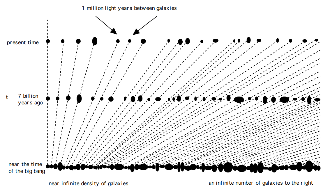
Figure \(\PageIndex{5}\): Even in the case of a universe that always was of infinite size, one can see an infinitely dense early universe by projecting present galactic density backward in time. (CC BY-NC-ND; Jack C. Straton)
For the k = 0 or k = −1 cases, we can again ask, “What is the universe expanding into?” Well, for these cases time is not synonymous with the radius of a sphere. In Figure \(\PageIndex{5}\), time points straight up and the galaxies are moving rightward. So the expansion is not into the future, nor does the universe create the universe it is expanding into. We can say, “The universe was already infinite at the start so there is plenty of universe for the universe to expand into, is there not?” This is best explicated by part of a story of two travelers checking into a hotel, modeled on David Hilbert’s ideas of infinity:
“We’re completely full, sir. Not even a dog kennel to spare. In fact, the dog seems to have doublebooked his kennel to a pack of huskies.”
Smith gestured at their huge pile of luggage. “Well, we’re not equipped for camping on the beach. We’ve got to stay somewhere!”
The receptionist nodded in sympathy. “Mmm, . . . I’ve got an idea, sir. But it will mean a bit of disruption . . . Let me check with the Manager.” She hurried off. About ten minutes later she returned, smiling broadly. “You’re in luck, Room 1 has just become vacant.”
“Brilliant.” A thought occurred to Smith. “Where are they going, then? You said the airport’s closed.”
“Into Room 2.”
“But Room 2 is occupied.”
“No, they’re moving into Room 3.”
“And where are they going?”
“Room 4, of course. We’ve relocated the people in Room 4 to Room 5. In fact, we’ve moved everybody up one room number.”
Smith felt his head spinning. “But . . . but what about whoever’s in the last room?”
“Ah, I see you’re labouring under a misconception. This is a Hilbert Hotel. There is no last room. We have infinitely many rooms—1, 2, 3, and so on forever. Right now, of course, they’re all full because we have infinitely many guests. But infinity plus one is still infinity, so we can rearrange the guests to create an extra room for you.”*
Thus, the answer to our question is tied up with the question of just which universe we are living in and does not seem to be answerable apart from that.
Note
* Ian Stewart, New Scientist 160, 58 (1998).
COSMIC INFLATION
In 1964, Peter W. Higgs proposed a mechanism to account for the existence of massive particles arising from the massless ones so far predicted by our theories.† One might roughly think of this Higgs field permeating all space acting as a drag on the motions of particles, making them more ponderous, as we are when we are walking in a swimming pool. Carl Hagen, Gerald Guralnik, and Tom Kibble also published a paper a month later on this topic.‡ Francois Englert and his colleague Robert Brout, who died in 2011, actually published their version two months before the publication of Higgs’s paper.§ But Higgs was the only one of the six who explicitly suggested that a particle would be associated with this field, whose spin would be zero (a class of particles known as bosons),¶ so his name was attached to that particle and via that to the field.
The Higgs boson was confirmed on July 4, 2012, at the CERN particle accelerator.** In 2013, Higgs and Englert were jointly awarded the Nobel Prize in Physics for their theories. (The rules of the Nobel stipulate that recipients be living persons, excluding Brout, and going to a maximum of three recipients, preventing the trio of Hagen, Guralnik, and Kibble from being added. In 2010, all six were awarded the J. J. Sakurai Prize for Theoretical Particle Physics.)
Note
† Peter W. Higgs, Phys. Lett. 12, 132 (1964); Phys. Rev. Lett. 13, 508 (1964).
‡ G. S. Guralnik, C. R. Hagen, and T. W. B. Kibble, Phys. Rev. Lett. 13, 585 (1964).
§ F. Englert and R. Brout, “Broken Symmetry and Mass of Gauge Vector—Mesons,” Phys. Rev. Lett. 13, 321 (1964).
¶ See “Interview to Prof. Peter Higgs About the Latest Results on the Searches for the Higgs Boson at the LHC,” CERN, July 4, 2012, http://cds.cern.ch/record/1459437.
** “New Results Indicate That Particle Discovered at CERN Is a Higgs Boson,” CERN, March 14, 2013, http://press.web .cern.ch/press-releases/2013/03/new-results-indicate-particle-discovered-cern-higgs-boson.
What would be the effect on the evolution of the Big Bang if there were a Higgs field permeating all space? In 1981, Alan Guth suggested that such a field would have a profound effect on the early expansion of the universe:* the negative pressure of the Higgs field would produce a repulsive gravitational force that would overpower its own inward tugging on spacetime once the density of the universe became low enough. Within 10−35 seconds the universe would double 100 times to become 1030 times its original size!† Andreas Albrecht with Paul Steinhardt and Andrei Linde, proposed modifications that account better for the production of a hot fireball at the end of this inflationary expansion that would look very much like the standard Big Bang.‡
Note
* Alan H. Guth, Phys. Rev. 23, 347 (1981).
† Alan H. Guth, The Inflationary Universe: The Quest for a New Theory of Cosmic Origins (Addison Wesley, Reading, MA, 1997), p. 171–77.
‡ Andreas Albrecht and Paul J. Steinhardt, Phys. Rev. Lett. 48, 1220 (1982); Andrei D. Linde, Phys. Lett. B 175, 395 (1986).
WHY WOULD THE HIGGS FIELD PRODUCE A NEGATIVE PRESSURE, AND WHY WOULD THIS OPPOSE GRAVITY?
One of the fascinating facets of quantum mechanics is Heisenberg’s uncertainty principle, which says that one cannot know both a particle’s position and its momentum with absolute certainty. Imagine, for instance, shining light on a tiny particle so that one may see it in a microscope. One would like to use light with a short wavelength, since objects have to be bigger than, or roughly the same size as, the distance between light wave crests in order to be seen. But unfortunately, short wavelength light, such as ultraviolet (UV) radiation, has higher energy and momentum* than long wavelength light, such as infrared (IR) light. So imaging the particle with UV would allow one to see where the particle is more easily, except that UV will also kick it away from the light source so that one has less of an idea of where it is after the attempt. On the other hand, imaging the tiny particle with IR would help keep the particle more in place while we image it, but IR waves are so long that we cannot use them to see the particle if that particle is small enough. This difficulty is a physical manifestation of the uncertainty principle.
Given that energy and time are related in relativity to momentum and position, one should not be surprised that an uncertainty principle involving time and energy also appears in quantum mechanics. One of the most interesting manifestations of this is that one may violate our certainty that energy is conserved as long as one does so for a very short time. It turns out that what we think about as the emptiness of spacetime constantly has pairs of electrons and their antimatter partners, called positrons, springing into existence, existing for a very short time, and then annihilating each other, giving back the energy they “borrowed” from the universe in order to come into being. Virtual protons and antiprotons likewise spring into existence in empty space, in the room before us, and in between our ears and live for a short enough time, within the uncertainty principle, that they do not ultimately violate energy conversation.
Dutch physicist Hendrik Casimir† predicted in 1948 that if one were to put two uncharged metal plates close enough together, the larger varieties of virtual particle pairs that can spring into being outside the plates, compared to those that can in between them, will tend to push the plates together. This prediction was confirmed in 1997 by S. K. Lamoreaux.‡ The vacuum is, thus, not empty at all; it has energy.
Note
* Yes, massless particles have momentum. In general, the ratio of momentum to energy is, from figure 3 of chapter 2, \(\frac{p}{E}=\frac{m v \gamma}{m c^{2} \gamma}=\frac{v}{c^{2}}\). For light, v = c so \(\frac{p}{E}=\frac{c}{c^{2}}=\frac{1}{c}\) or p = E/c.
† H. B. G. Casimir, Proc. K. Ned. Akad. Wet. 51, 793 (1948).
‡ S. K. Lamoreaux, Phys. Rev. Lett. 78, 5 (1997).
SYMMETRY BREAKING
In 1918, a German mathematician named Emmy Noether discovered and published what is the most profound theorem on symmetry to date. She gave us a relation between symmetries and conservation laws. A spinning ice skater who pulls her arms in speeds up. Why is this? She has angular momentum as she spins, which is a product of her mass, the speed of her spin, and the distance of her mass from the spin axis. As she pulls her arms in, the distance of part of her mass from the spin axis decreases, and the only thing one may balance this change with to keep her angular momentum constant is to speed her up.
But there is a deeper why to this. Noether showed that angular momentum conservation is a consequence of the symmetry (angular uniformity) of the space surrounding the skater. She showed that if you turn through an infinitesimal angle, the difference of kinetic and potential energies—which is called the Lagrangian—is unchanged. By adding up a bunch of zero changes for a bunch of these tiny angles, she showed that the Lagrangian is unaffected by any rotation of the entire system in a uniform space. If, on the other hand, an ice skater spinning to face a more northerly direction encountered a space that somehow made her more sluggish than spinning to face a more southerly direction, the Lagrangian would not be symmetrical and her angular momentum would not be conserved.
Linear momentum conservation is a consequence of the uniformity of space before you (ignoring trees and rocks and such), and energy conservation is a consequence of the uniformity of the flow of time. High energy physicists have applied Noether’s theorem to every Lagrangian they can find a symmetry for, many of which have nothing to do with space or time.
What does this mean for the Higgs field? Consider again Figure \(\PageIndex{6}\) of chapter 4, which modeled the transformation of potential energy into kinetic energy. We can also think of that figure as portraying a more abstract concept, symmetry. A marble rolling in the bowl has no preference for the left rim or the right; it just rolls back and forth. Likewise, an iron magnet that is heated above the Curie temperature,‡ 770° C, loses its magnetization; the magnetic moment vectors of the bar’s electrons are equally likely to be aligned toward the left as toward the right.
Actually, the ball in the bowl would be equally content to roll in the forward and backward directions as left and right. If we were to start its motion at any point around the rim, nothing changes in its oscillatory motion since the bowl is rotationally symmetrical. Given a bit of friction, the ball will eventually come to rest at the lowest potential energy position, in the center. In the case of electrons, the point of zero magnetization corresponds to what we call the ground state or vacuum state.
The potential energy curve for the bar magnet at high temperatures is likewise rotationally symmetrical; the magnetic moment vectors of the bar’s electrons could point in any direction. But as the temperature drops below 770° C, the potential energy curve for the bar magnet slumps to the left and the right of the central vacuum state, as in Figure \(\PageIndex{6}\) of the present chapter. A ball rolling in this shape of a bowl would come to rest in the newly created trough at some point away from the central peak. It might be to the right or to the left or to the front or the back of the central peak, but it will be in a definite direction.
There is no one who chooses this final position so we say that the rotational symmetry is “spontaneously broken,” replaced with a lesser symmetry called parity, in which the ball’s position relative to the central peak in Figure \(\PageIndex{6}\) will look the same to us if we see it reflected in a mirror lying in the same plane as this page. The magnetic moment vectors of the bar’s electrons will point to one position—for instance, to the right in Figure \(\PageIndex{6}\). The bar magnet will, in this case, have its north magnetic pole to the right and its south magnetic pole to the left.
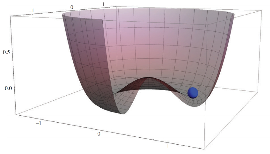
Note that the vacuum state of the bar magnet is generally in one of these trough positions, such as to the right in Figure \(\PageIndex{6}\), and not in the state of zero magnetization at the center of what has come to be a peak. But there is a slight chance that should the “ball” be at rest in the center of the high-temperature bowl shape as the temperature drops, it could stay at rest at this point that becomes the peak as the bowl slumps on either side of it, though the slightest “breeze” or other perturbation would knock it off. We would say that the ball at rest on the peak would then be in a “false vacuum” state, because this is not the lowest-energy state of the system. The ball would be in an unstable position and the slightest disturbance would cause it to roll off the peak and down into the trough.
Note
‡ Named after Marie Curie’s husband, Pierre.
BREAKING THE HIGGS SYMMETRY
This discussion of symmetry breaking as temperature falls when the universe expands applies as well in the case of the Higgs fields, with two crucial twists in the story. As Guth first proposed it, the central peak that develops in Figure \(\PageIndex{6}\) has a dimple in it that would allow the universe (the ball) to remain at that central position as the universe cools. (The models of Linde and of Albrecht and Steinhardt have a very broad plateau, instead of a dimple, that nevertheless lets the universe stay in the false vacuum state for a long time before it “rolls off.”) The consequences of this are profound.
A photon is a bundle of energy whose energy is contained in oscillations in its electric and magnetic fields. If one were to put photons in a piston with reflective walls and pull the plunger outward, the energy per unit volume—the energy-density—would diminish as the oscillations spread out in the larger volume. The same argument holds for the quantum fields associated with material particles like electrons. These sorts of particles will shove outward on the plunger as they ricochet around inside the piston. They will exert pressure. Were you to have your hand on the piston, you would have to resist its movement outward, just as you need to hold down the lid of a popcorn popper as it is randomly knocked upward by exploding kernels.
The latter analogy helps us understand what keeps a star from collapsing under its own weight: the balancing of gravity by the outward pressure of extremely hot gasses ricocheting off each other, as we discussed in the last chapter. But there is a subtlety in this balancing the inward gravitational force with the outward heat pressure if we move from the Newtonian idea of gravitational force to the Einsteinian warpage of spacetime. Just like mass and energy, pressure is a quantity that causes spacetime to warp downward into the time direction. That is, the pressure that keeps a star’s gasses from collapsing inward—from rolling down that funnel toward its center—also causes a deeper funnel that will cause gasses to more readily roll down that slope toward its center. This snake eating its tail in Einstein’s theory of gravity is what makes the equations so difficult to solve for specific problems. But given the right resources, one can show that there will nevertheless be some size for the star at which the inward and outward tendencies on the gasses do balance.
Suppose we were to try to contain the false vacuum associated with the Higgs field in a piston. Unlike that of photons or conventional particles, the energy of the Higgs field is not contained in any oscillations of this field but in a number, in the value of the Higgs field. So its energy-density is constant. As one pulls the plunger outward on this piston, the volume of the false vacuum increases, and since its energy per unit volume is constant, the energy inside the piston must increase. Where would this energy come from? It would be provided by your hand pulling outward on the plunger. Put another way, should you attempt to pull outward on the plunger, you will feel a resistance from the false vacuum inside. Unlike a piston filled with conventional gasses or particles, the Higgs vacuum exerts negative pressure.
So what do you suppose is the gravitational effect of this negative pressure if the gravitational effect of conventional, positive pressure is a stronger gravitational force or a deeper warpage of spacetime downward? Indeed, it would be a warpage of spacetime upward that will send objects rolling outward rather than inward. In Newtonian terms, the negative pressure of the expanding Higgs false vacuum will exert an antigravitational force. Our positive pressure holding up a star caused more gravitational force inward that moved the gasses inward until they experienced even more positive pressure to balance it. Likewise, the antigravitational force caused by the negative pressure of the Higgs false vacuum would cause it to expand further and this would exert a larger antigravitational force. This leads to a runaway expansion of epic proportions. Within 10−35 seconds, the universe would double 100 times to become 1030 times its original size!*
Note
* Alan H. Guth, The Inflationary Universe: The Quest for a New Theory of Cosmic Origins (Addison Wesley, Reading, MA, 1997), p. 171–77.
IS THERE EVIDENCE OF INFLATION?
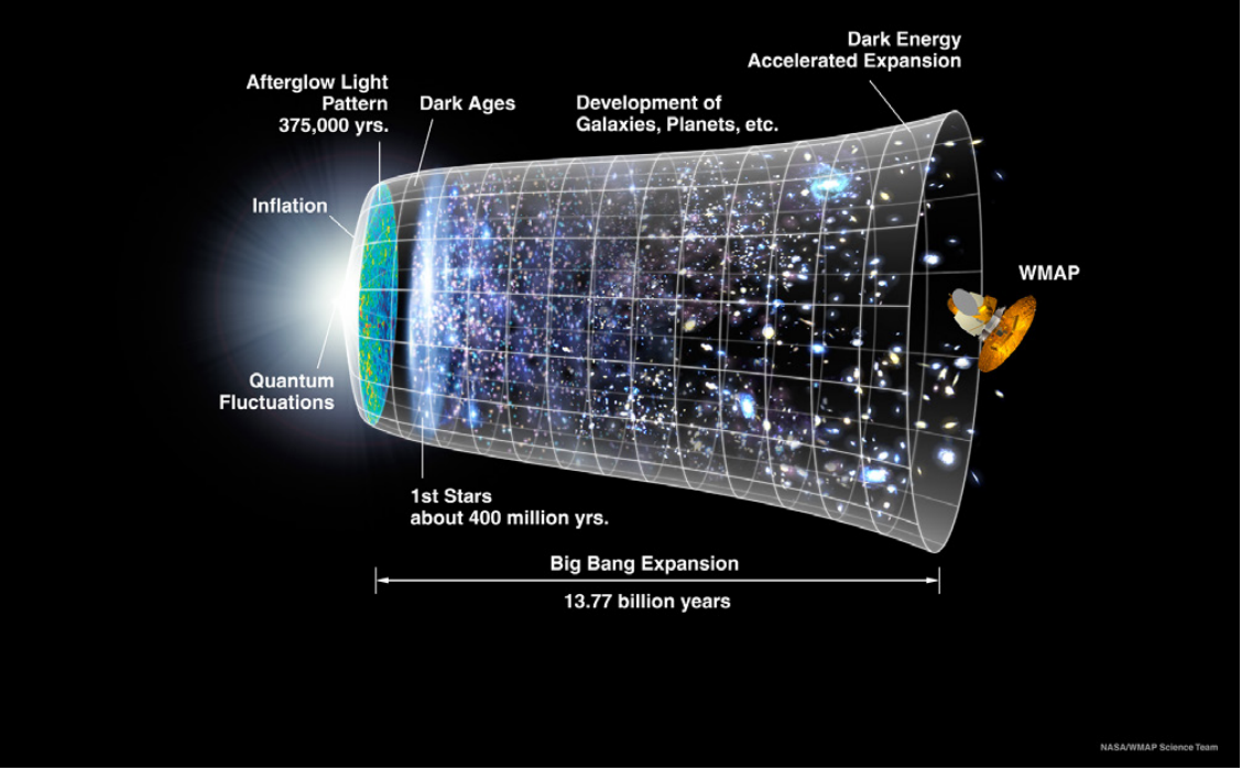
A diagram reproduced in Figure \(\PageIndex{7}\), from the Wilkinson Microwave Anisotropy Probe (WMAP) mission, shows the initial inflationary fraction of a second on the left, a standard Big Bang expansion in the middle, and an accelerating expansion (which we will get to in a bit) on the right.
Note
* NASA/WMAP Science Team, “Timeline of the Universe,” National Aeronautics and Space Administration, last modified December 21, 2012, https://map.gsfc.nasa.gov/media/060915/index.html.
Given the enormous rate of expansion in the inflationary period, if the universe has a spherical shape, the current radius of the universe should be so large that it would appear flat to us, as ants walking on the surface of the US Capitol dome would perceive it to be. Inflationary expansion would also drive an originally saddle-shaped universe to be flat. If it were originally flat, it would remain so.
If we look at the map of the radiation left over from the Big Bang, the “afterglow light pattern” at 370,000 years, labeled as such in time in Figure \(\PageIndex{7}\) and fully shown in Figure \(\PageIndex{8}\), we see that this Cosmic Microwave Background (CMB) radiation, as it is more conventionally called, has fluctuations in temperature in the fifth decimal place and fluctuations in brightness: “If the universe were flat, the brightest microwave background fluctuations (or ‘spots’) would be about one degree across. If the universe were open, the spots would be less than one degree across. If the universe were closed, the brightest spots would be greater than one degree across.” WMAP has confirmed that the brightest spots are indeed about one degree across. As of 2013, WMAP tells us that “the universe is flat with only a 0.4% margin of error [and] that the Universe is much larger than the volume we can directly observe.”*
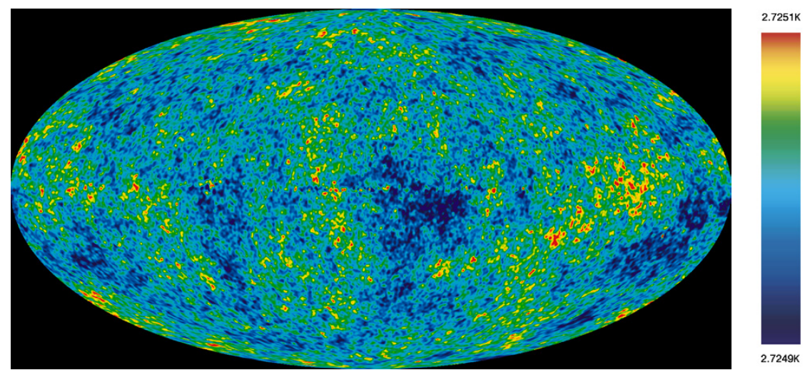
Inflation also accounts for why regions of the universe far to the left and far to the right are at the same temperatures to five decimal places in Figure \(\PageIndex{8}\). They are so far apart that energy in the form of light could not have traveled between them to equalize their temperatures within the 13.77 billion years WMAP data says is the age of the universe. However, their having nearly equal temperatures today would be what we would expect if their temperatures had been equalized when they were infinitesimal distances apart from each other in the early stages of universal expansion and then were flung far apart by inflation.
As a side note, it has been suggested that an inflationary expansion would magnify the spacetime foam shown in Figure \(\PageIndex{11c}\) of chapter 4 to such an extent that we should see huge voids of nothingness between today’s clusters of galaxies. Indeed, that is what Margaret J.
Note
* NASA/WMAP Science Team, “Will the Universe Expand Forever?,” National Aeronautics and Space Administration, last modified January 24, 2014, https://map.gsfc.nasa.gov/universe/uni_shape.html.
† NASA/WMAP Science Team, “CMB Images,” National Aeronautics and Space Administration, last modified April 14, 2014, https://map.gsfc.nasa.gov/media/121238/index.html.
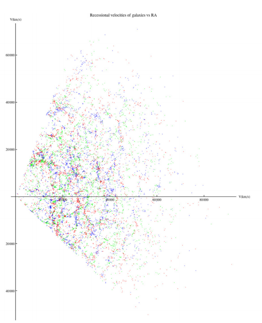
Geller and John P. Huchra found by mapping the distribution of galaxies.* The reader may measure the red-shift velocities of some 200 galaxies in a telescope simulator called CLEA, available from Gettysburg College,† and plot this information against their angular positions (called right ascension [RA] and equivalent to longitude on the Earth’s surface) in a small slice of the other angle (called declination [Dec.] and equivalent to latitude). Even with just 200 galaxies, the bubble structure is apparent, and it grows more marked with larger numbers of galaxies and adjacent declinations.
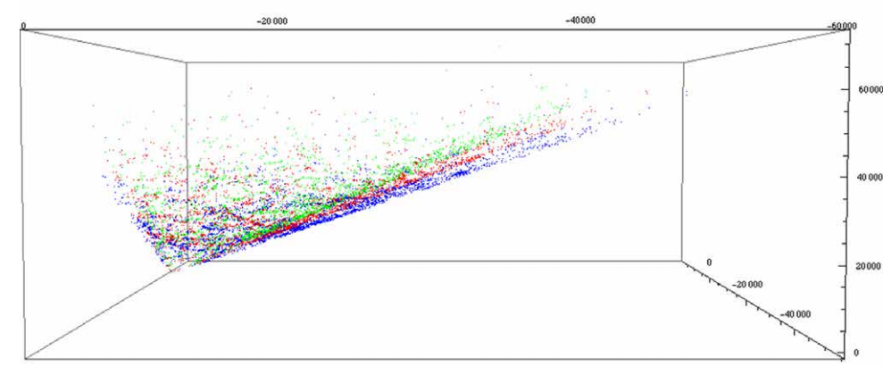
Those desiring to plot thousands of galaxies may access the Las Campanas Redshift Survey Catalog,‡ the results of which are shown in Figure \(\PageIndex{10}\). This is a composite of a trio of three-degree slices of the sky that one may see stacked not quite edge-on in Figure \(\PageIndex{9}\) as red, green, and blue fans of galaxies.
Note
* M. J. Geller and J. P. Huchra, Science 246, 897 (1989).
† The original Windows version is at http://www3.gettysburg.edu/~marschal/clea/univlab.html, and the version bottled for Macintosh by Joel Cranston is at http://archives.pdx.edu/ds/psu/15113.
‡ In the search page at https://heasarc.gsfc.nasa.gov/db-perl/W3Browse/w3table.pl?tablehead=name%3Dlcrscat&Action= More+Options, one types “−46 .. −44” in the “dec” box and “> 1045” in the “radial velocity” box and hits “Start Search.” The automatic result is to limit the search to 1,000 galaxies. One may then change “Maximum Rows”: to “4,000” and hit the “Reissue Query” button. I changed the download from the default “Tabbed” to “Excel-compatible” and saved the file. I rearranged the columns so that “ra,” “dec,” and “radial_velocity” were in columns a, b, and c, and in cell K2 entered the equation “= “{“&RADIANS(A2)&”,”&C2&”},”.” I filled down to cell K4001 and copied the results into a Mathematica notebook. The four-term version would read "\(\mathrm{k} 45:=\{\{1.20937371982484,31150\},\{1.09713211922786,36760\},\{1.11332964735099,42616\},\{0.989954765988463,13140\}\}\)," where I have replaced the last comma with a curly bracket. The Mathematica instruction, “ListPolarPlot[k45, PlotStyle −> Directive[PointSize[Tiny], Magnification −> 0.1, Blue]]” gives the blue plot.
WHICH UNIVERSE DO WE LIVE IN?
The debate for 75 years had been whether the universe would slow its expansion but continue to expand forever or eventually stop and begin contracting into a Big Crunch. In 1998, two teams observing the brightness of distant Type Ia supernovae (stellar explosions of known intrinsic luminosity) independently determined that the expansion of the universe is actually accelerating.* (The team leaders—Adam Riess, Brian Schmidt, and Saul Perlmutter—were awarded the 2011 Nobel Prize in Physics for their discovery.) See the right-hand side of Figure \(\PageIndex{7}\).
What is causing this acceleration? This substance, which has to make up for 71.4% of the energy of the universe to account for current WMAP observations of the light left over from the Big Bang,† has been dubbed Dark Energy, but no one really knows what it is. Another 24% of the energy of the universe is dark matter, whose composition is likewise unknown and interacts with conventional matter (4.6% of the energy of the universe) only gravitationally.
Dark matter was first suggested by Fritz Zwicky as a way to explain the observed motions of galaxies in the Coma cluster of galaxies: “[T]he average density in the Coma system would have to be at least 400 times greater than that derived on the basis of observations of luminous matter.”‡ Vera C. Rubin and W. Kent Ford’s measurement of the flat rotational speed curves of regions in the Andromeda Galaxy in 1970, and subsequently many other galaxies, provided sufficient evidence that dark matter extended far beyond the optically bright edge of galaxies to make the assumption of its existence the norm within astronomy.§
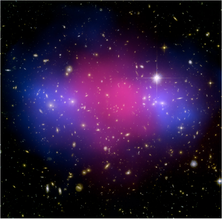
Figure \(\PageIndex{11}\) is a composite image: the Hubble space telescope was used to map the dark matter (colored in blue) using a technique known as gravitational lensing. Chandra X-ray Observatory’s data enabled the astronomers to accurately map the ordinary matter, mostly in the form of hot gas, which glows brightly in X-rays (shown in pink). It is significant that the blue lobes on either side, consisting of dark matter, have passed through the pink collision region with little to no interaction with the conventional matter. Indeed, there was little to no interaction with the oncoming dark matter from the other galaxy cluster other than the gravitational interaction that will eventually pull both ordinary matter and dark matter components into a rough ball in the central region.
Note
* Adam G. Riess et al., Astron. J. 116, 1009 (1998), http://iopscience.iop.org/1538-3881/116/3/1009/fulltext/; Astrophys. J. 517, 565 (1999), http://iopscience.iop.org/0004-637X/.../565/fulltext/.
† NASA/WMAP Science Team, “Universe Content—WMAP 9yr Pie Chart,” National Aeronautics and Space Administration, last modified April 8, 2014, https://map.gsfc.nasa.gov/media/121236/index.html.
‡ Fritz Zwicky, Helvetica Physica Acta 6, 110 (1933), with an English translation by Heinz Andernach at https://arxiv.org/abs/1711.01693. See section 5.
§ Vera C. Rubin and W. Kent Ford Jr., Astrophys. J. 159, 379 (1970).
Note
* NASA Science Team, “A Clash of Clusters Provides Another Clue to Dark Matter,” National Aeronautics and Space Administration, August 27, 2008, https://www.nasa.gov/mission_pages/c...tos08-111.html. See also the Bullet Cluster: “1E 0657-56: NASA Finds Direct Proof of Dark Matter,” National Aeronautics and Space Administration, last modified August 27, 2018, http://chandra.harvard.edu/photo/2006/1e0657/.
One theory is that Dark Energy is what is known as the cosmological constant, a fudge factor Λ that Einstein added to his theory in 1917 to prevent an outward expansion and, thus, to match what nearly everyone believed was a static universe. He later told George Gamow “that the introduction of the cosmological term was the biggest blunder he ever made in his life.”*
There is a second Friedmann equation† that gives the acceleration, A, of the universe, defined as the change in the speed of expansion, S, with time,
\[A=-\frac{4 \pi G}{3} \rho+\frac{3}{c^{2}} p R \tag{5}\]
where \(\rho\) is the conventional and dark matter density and p is the pressure of the universe. Einstein had wanted a static universe, one that did not change speed, so he would need A = 0. The most obvious ways one could do that is to have both \(\rho\) and p = 0 or R = 0. But the first idea is no good because this is a universe with nothing in it. The second is no better since it constitutes no universe to speak of. The better solution that apparently came to Einstein was to postulate a substance pervading the universe that has negative pressure of just the right size that the term in parentheses in Equation (5) is 0. That is, at the present moment in time,
\[A_{0}=-\frac{4 \pi G}{3} \rho_{0}+\frac{3}{c^{2}} p_{0} \quad R_{0}=-\frac{4 \pi G}{3} \rho_{0}+\frac{3}{c^{2}}-\rho_{0} \frac{c^{2}}{3} \quad R_{0}=0 \tag{6}\]
This solution saw the light of day for only a few years before observations showed that the universe was expanding, undermining the need for a static solution.
Although this solution seems to do what Einstein wanted, it is highly unstable. If the universe were to shrink ever so slightly, the matter density would increase by a tiny factor, but the negative pressure of the substance pervading all space would not change. This increase in the matter density would pull the matter further inward, again increasing the matter density, and so on, and one would ultimately have a runaway collapse of the universe.
Or if the universe were to expand ever so slightly, the matter density would decrease by a tiny factor but the negative pressure of the substance pervading all space would not change. This disbursement of the matter to a larger volume would have less of an inward gravitational tug, allowing the matter to move farther apart, again decreasing the matter density, and so on, and one would ultimately have a runaway expansion of the universe. Although this instability would have proved a disaster for Einstein’s attempt at finding a static solution for the universe, it is just what one needs for a runaway expansion of the universe like that observed in 1998.
Note
* George Gamow, My World Line, an Informal Autobiography (Viking Press, New York, 1970), p. 44.
† Tai L. Chow, Gravity, Black Holes, and the Very Early Universe an Introduction to General Relativity and Cosmology (Springer, New York, 2008), p. 142, eq. (8.36–37).
In this case, we want a version of Equation (6) whose acceleration, radius, and mass density can change with time. Also, the negative pressure (the interior parenthesis on the right-hand side of Equation [6]) is more conventionally written in terms of the cosmological constant, Λ, so we transform Equation (6) to read
\[A=-\frac{4 \pi G}{3} \rho R+\frac{4 \pi G \rho_{0}}{3} R \equiv-\frac{4 \pi G}{3} \rho R+\frac{\Lambda}{3} R \tag{7}\]
The required “substance” with negative pressure could simply be the vacuum energy of “empty” space Casimir’s work led us to.
This adds a new term to Equation (4a), the first Friedmann equation that gives the expansion velocity of the universe:
\[S^{2} / c^{2}=R_{\max } / R-k+1 / 3 \ \Lambda \ R^{2} / c^{2} \tag{8a}\]
One sees that early enough in the expansion of the universe, R is small, and its square is smaller still, so that Λ will have no discernible effect. But eventually, R will get big enough and its square will drive the expansion speed S to larger and larger values. This first Friedmann equation, too, gives a runaway acceleration of the universe that is just starting in the visualization Equation (8b) with k = 1,
There are candidates for what is driving the acceleration of the universe other than the vacuum energy of “empty” space, and there also are some unresolved problems with calculating the vacuum energy density. See, for instance, the work of Robert Caldwell, Rahul Dave, and Paul Steinhardt on a form of dark energy called “quintessence.”* We will leave readers to explore such on their own—after, of course, listening to some more music, say Youssou N’Dour’s song “Liggey” (Live In London, 2003).
Note
* R. R. Caldwell, R. Dave, and P. J. Steinhardt, Phys. Rev. Lett. 80 (8), 1582–85 (1998).