7.6: Volume, Orientation, and the Levi-Civita Tensor

Learning Objectives

• Introduction of some geometrical machinery that is used in both special and general relativity

This optional section introduces some geometrical machinery that is used in both special and general relativity.

Volume

Desirable properties

In \(3 + 1\) dimensions, we have a natural way of defining four dimensional volume, which is to pick a frame of reference and let the element of volume be \(dt dx dy dz\) in the Minkowski coordinates of that frame. Although this definition of \(4\)-volume is stated in terms of certain coordinates, it turns out to be Lorentz-invariant (section 2.5). It also has the following desirable properties, which we state for an arbitrary value of \(m\) from \(1\) to \(4\):

1. V1. Any two \(m\)-volumes can be compared in terms of their ratio.
2. V2. For any \(m\) nonzero vectors, the \(m\)-volume of the parallelepiped they span is nonzero if and only if the vectors are linearly independent (that is, if none of them can be expressed in terms of the others using scalar multiplication and vector addition).

We would also like to have convenient methods for working with three-volume, two-volume (area), and one-volume (length). But the \(m\)-volumes for \(m < 4\) give us headaches if we try to define them so that they obey both V1 and V2. For example, the obvious way to define length (\(m = 1\)) is to use the metric, but then lightlike vectors would violate V2.

Affine measure

If we’re willing to abandon V1, then the following approach succeeds. Consider the \(m = 1\) case. We ignore the metric completely and exploit the fact that in special relativity, spacetime is flat (postulate P2), so that parallelism works the same way as in Euclidean geometry. Let \(l\) be a line, and suppose we want to define a number system on this line that measures how far apart events are. Depending on the type of line, this could be a measurement of time, of spatial distance, or a mixture of the two.

Figure \(\PageIndex{1}\): Using parallelism to define 1-volume.

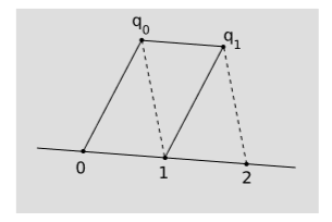
First we arbitrarily single out two distinct points on \(l\) and label them \(0\) and \(1\), as in figure \(\PageIndex{1}\). Next, pick some auxiliary point \(q_0\) not lying on \(l\). Construct \(q_0 q_1\) and parallel to \(01\) and \(1q_1\) parallel to \(0q_0\), forming the parallelogram shown in the figure. Continuing in this way, we have a scaffolding of parallelograms adjacent to the line, determining an infinite lattice of points \(1, 2, 3, ...\) on the line, which represent the positive integers. Fractions can be defined in a similar way. For example, \(\tfrac{1}{2}\) is defined as the point such that when the initial lattice segment \(0\tfrac{1}{2}\) is extended by the same construction, the next point on the lattice is \(1\). The continuously varying variable constructed in this way is called an affine parameter. The time measured by a freefalling clock is an example of an affine parameter, as is the distance measured by the tick marks on a free-falling ruler. An affine parameter can only be defined along a straight world-line, not an arbitrary curve. The affine measurement of \(1\)-volume violates V1, because it only allows us to compare distances that lie on \(l\) or parallel to it. On the other hand, it has the advantage over metric measurement that it allows us to measure lengths along lightlike lines.

Figure \(\PageIndex{2}\): The area of the viola can be determined by counting the parallelograms formed by the lattice. The area can be determined to any desired precision, by dividing the parallelograms into fractional parts that are as small as necessary.

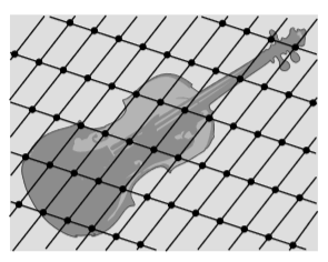
Figure \(\PageIndex{2}\) shows how to define an affine measure of \(2\)-volume, and a similar method works for \(3\)-volume.

Linearity

Figure \(\PageIndex{3}\): Linearity of area. Doubling the vector a doubles the area.

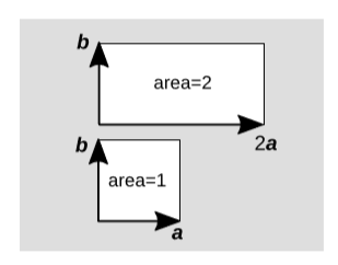
Suppose that a parallelogram is formed with vectors a and b as two of its sides. It we double a, then the area doubles as well,

\[area(2a,b) = 2area(a,b)\]

In general, if we scale either of the vectors by a factor \(c\), the area scales by the same factor, provided that we set some rule for handling signs — an issue that we’ll postpone until the Orientation section below. Something similar happens when we add two vectors, e.g.,

\[area(a,b + c) = area(a,b) + area(a,c)\]

again postponing issues with signs. We refer to these properties as linearity of the affine \(2\)-volume. Any sensible measure of m-volume should have similar linearity properties.

Change of basis

Figure \(\PageIndex{4}\): The viola has a different area when measured using a different parallelogram as the unit.

Because we have not made use of the metric so far, all of our measures of area have been relative rather than absolute. As shown in figure \(\PageIndex{4}\), they depend on what parallelogram we choose as our unit of area. The unit cell in figure \(\PageIndex{4}\) (2) is smaller than the one in figure \(\PageIndex{1}\) (1), for two reasons: the vectors defining the edges are shorter, and the angle between them is smaller. Words like “shorter” and “angle” show us resorting to metric measurement, but we could also perform the comparison without using the metric, simply by using parallelogram \(1\) to measure parallelogram \(2\), or \(2\) to measure \(1\). If we think of such a pair of vectors as basis vectors for the plane, then switching our choice of unit parallelogram is equivalent to a change of basis. Areas change in proportion to the determinant of the matrix specifying the change of basis.

Example \(\PageIndex{1}\): A halFLing basis

Suppose that \(a' = a/2\), and \(b' = b/2\). The change of basis from the unprimed pair to the primed pair is given by the matrix

\[\begin{pmatrix} 2 & 0\\ 0 & 2 \end{pmatrix}\]

which has determinant \(4\). Scaling down both basis vectors by a factor of \(2\) has caused a reduction by a factor of \(4\) in the area of the unit parallelogram. If we use the primed parallelogram to measure other areas, then all the areas will come out bigger by a factor of \(4\).

Rotations and Lorentz boosts are changes of basis. They have determinants equal to \(1\), i.e., they preserve spacetime volume.

Orientation

Figure \(\PageIndex{5}\): Linearity of area requires that some areas be assigned negative values.

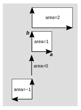
As shown in figure \(\PageIndex{5}\), linearity of area requires that some areas be assigned negative values. If we compare the areas \(+1\) and \(-1\), we see that the only difference is one of orientation, or handedness. In the case to which we have arbitrarily assigned area \(+1\), vector b lies counterclockwise from vector a, but when a is flipped, the relative orientation becomes clockwise.

If you’ve had the usual freshman physics background, then you’ve seen this issue dealt with in a particular way, which is that we assume a third dimension to exist, and define the area to be the vector cross product \(a×b\), which is perpendicular to the plane inhabited by \(a\) and \(b\). The trouble with this approach is that it only works in three dimensions. In four dimensions, suppose that a lies along the \(x\)-axis, and \(b\) along the \(t\)-axis. Then if we were to define \(a×b\), it should be in a direction perpendicular to both of these, but we have more than one such direction. We could pick anything in the \(y-z\) plane.

To get started on this issue in m dimensions, where \(m\) does not necessarily equal \(3\), we can consider the \(m\)-volume of the \(m\)-dimensional parallelepiped spanned by \(m\) vectors. For example, suppose that in \(4\)-dimensional spacetime we pick our \(m\) vectors to be the unit vectors lying along the four axes of the Minkowski coordinates, \(\hat{t},\hat{x},\hat{y}\; \text{and}\; \hat{z}\). From experience with the vector cross product, which is anticommutative, we expect that the sign of the result will depend on the order of the vectors, so let’s take them in that order. Clearly there are only two reasonable values we could imagine for this volume: \(+1\) or \(-1\). The choice is arbitrary, so we make an arbitrary choice. Let’s say that it’s \(+1\) for this order. This amounts to choosing an orientation for spacetime.

A hidden and nontrivial assumption was that once we made this choice at one point in spacetime, it could be carried over to other regions of spacetime in a consistent way. This need not be the case, as suggested in figure \(\PageIndex{6}\).

Figure \(\PageIndex{6}\): A Möbius strip is not an orientable surface.

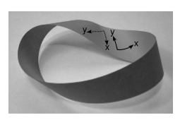
However, our topic at the moment is special relativity, and as discussed briefly in section 2.4, it is usually assumed in special relativity that spacetime is topologically trivial, so that this issue arises only in general relativity, and only in spacetimes that probably are not realistic models of our universe.

Since \(4\)-volume is invariant under rotations and Lorentz transformations, our choice of an orientation suffices to fix a definition of \(4\)-volume that is a Lorentz invariant. If vectors \(a\), \(b\), \(c\), and \(d\) span a \(4\)-parallelepiped, then the linearity of volume is expressed by saying that there is a set of coefficients \(\epsilon _{ijkl}\) such that

\[V = \epsilon _{ijkl} a^i b^j c^k d^l\]

Notating it this way suggests that we interpret it as abstract index notation, in which case the lack of any indices on \(V\) means that it is not just a Lorentz invariant but also a scalar.

Example \(\PageIndex{2}\): HaLFLing coordinates

Let \((t,x,y,z)\) be Minkowski coordinates, and let \((t',x',y',z') = (2t,2x,2y,2z)\). Let’s consider how each of the factors in our volume equation is affected as we do this change of coordinates.

\[\overset{\underbrace{V}}{\text{no change}}\; \; = \; \; \overset{\underbrace{\epsilon _{\kappa \lambda \mu \nu }}}{\times 1/16}\; \overset{\underbrace{a^{\kappa }}}{\times 2}\; \overset{\underbrace{b^{\lambda }}}{\times 2}\; \overset{\underbrace{c^{\mu }}}{\times 2}\; \overset{\underbrace{d^\nu }}{\times 2}\]

Since our convention is that \(V\) is a scalar, it doesn’t change under a change of coordinates. This forces us to say that the components of change by a factor of \(1/16\) in this example.

The result of Example \(\PageIndex{2}\) tells us that under our convention that volume is a scalar, the components of must change when we change coordinates. One could argue that it would be more logical to think of the transformation in this example as a change of units, in which case the value of \(V\) would be different in the new units; this is a possible alternative convention, but it would have the disadvantage of making it impossible to read off the transformation properties of an object from the number and position of its indices. Under our convention, we can read off the transformation properties in this way. Although section 7.4 only presented these properties in the case of tensors of rank \(0\) and \(1\), deferring the general description of higher rank tensors to section 9.2, \(\epsilon\)’s transformation properties are, as implied by its four subscripts, those of a tensor of rank \(4\). Different authors use different conventions regarding the definition of \(\epsilon\), which was originally described by the mathematician Levi-Civita.

Figure \(\PageIndex{7}\): Tullio Levi-Civita (1873-1941) worked on models of number systems possessing infinitesimals and on differential geometry. He invented the tensor notation, which Einstein learned from his textbook. He was appointed to prestigious endowed chairs at Padua and the University of Rome, but was fired in 1938 because he was a Jew and an anti-fascist.

Since by our convention \(\epsilon\) is a tensor, we refer to it as the Levi-Civita tensor. In other conventions, where \(\epsilon\) is not a tensor, it may be referred to as the Levi-Civita symbol. Since the notation is not standardized, I will occasionally put a reminder next to important equations containing \(\epsilon\) stating that this is the tensorial \(\epsilon\).

The Levi-Civita tensor has lots and lots of indices. Scary! Imagine the complexity of this beast. (Sob.) We have four choices for the first index, four for the second, and so on, so that the total number of components is \(256\). Wait, don’t reach for the kleenex. The following example shows that this complexity is illusory.

Example \(\PageIndex{3}\): Volume in Minkowski coordinates

We’ve set up our definitions so that for the parallelepiped \(\hat{t},\hat{x},\hat{y},\hat{z}\), we have \(V = +1\). Therefore

\[\epsilon _{txyz} = +1\]

by definition, and because \(4\)-volume is Lorentz invariant, this holds for any set of Minkowski coordinates.

If we interchange \(x\) and \(y\) to make the list \(\hat{t},\hat{y},\hat{x},\hat{z}\), then as in figure \(\PageIndex{5}\), the volume becomes \(-1\), so

\[\epsilon _{tyxz} = -1\]

Suppose we take the edges of our parallelepiped to be \(\hat{t},\hat{x},\hat{x},\hat{z}\), with \(y\) omitted and \(x\) duplicated. These four vectors are not linearly independent, so our parallelepiped is degenerate and has zero volume.

\[\epsilon _{txxz} = 0\]

From these examples, we see that once any element of has been fixed, all of the others can be determined as well. The rule is that interchanging any two indices flips the sign, and any repeated index makes the result zero.

Example \(\PageIndex{3}\) shows that the the fancy symbol \(\epsilon _{ijkl}\), which looks like a secret Mayan hieroglyph invoking \(256\) different numbers, actually encodes only one number’s worth of information; every component of the tensor either equals this number, or minus this number, or zero. Suppose we’re working in some set of coordinates, which may not be Minkowski, and we want to find this number. A complicated way to find it would be to use the tensor transformation law for a rank-\(4\) tensor (section 9.2). A much simpler way is to make use of the determinant of the metric, discussed in Example 6.2.1. For a list of coordinates ijkl that are sorted out in the order that we define to be a positive orientation, the result is simply \(\epsilon _{ijkl} = \sqrt{\left | det\; g \right |}\). The absolute value sign is needed because a relativistic metric has a negative determinant.

Example \(\PageIndex{4}\): Cartesian coordinates and their halFLIng versions

Consider Euclidean coordinates in the plane, so that the metric is a \(2×2\) matrix, and \(\epsilon _{ij}\) has only two indices. In standard Cartesian coordinates, the metric is \(g = diag(1,1)\), which has \(det\; g = 1\). The Levi-Civita tensor therefore has \(\epsilon _{xy} = +1\]), and its other three components are uniquely determined from this one by the rules discussed in Example \(\PageIndex{3}\). (We could have flipped all the signs if we had wanted to choose the opposite orientation for the plane.) In matrix form, these rules result in

\[\epsilon = \begin{pmatrix} 0 & 1\\ -1 & 0 \end{pmatrix}\]

Now transform to coordinates \((x',y') = (2x,2y)\). In these coordinates, the metric is \(g' = diag(1/4,1/4)\), with \(det\; g = 1/16\), so that \(\epsilon _{x'y'} = 1/4\), or in matrix form,

\[\epsilon '= \begin{pmatrix} 0 & 1/4\\ -1/4 & 0 \end{pmatrix}\]

Example \(\PageIndex{5}\): Polar coordinates

In polar coordinates \((r,θ)\), the metric is \(g = diag(1,r^2)\), which has determinant \(r^2\). The Levi-Civita tensor is

\[\epsilon = \begin{pmatrix} 0 & r\\ -r & 0 \end{pmatrix}\]

(taking the same orientation as in Example \(\PageIndex{4}\)).

Example \(\PageIndex{6}\): Area of a circle

Let’s find the area of the unit circle. Its (signed) area is

\[A = \int \text{2-volume}(dr, d\theta )\]

where the order of \(dr\) and \(dθ\) is chosen so that, with the orientation we’ve been using for the plane, the result will come out positive. Using the definition of the Levi-Civita tensor, we have

\[\begin{align*} A &= \int \epsilon _{r\theta } dx^r dx^\theta \\ &= \int_{r = 0}^{1}\int_{\theta =0}^{2\pi }rdrd\theta \\ &= \pi \end{align*}\]

The 3-volume covector

Consider the volume of a three-dimensional subspace of four-dimensional spacetime. Linearity leads to an especially simple characterization of the \(3\)-volume. Let a \(3\)-volume be defined by the parallelepiped spanned by vectors \(a\), \(b\), and \(c\). If we threw in a fourth vector \(d\), we would have a \(4\)-volume, and \(4\)-volume is a scalar. This \(4\)-volume would depend in a linear way on all four vectors, and in particular it would depend linearly on \(d\). But this means we have a scalar that is a linear function of a vector, and such a function is exactly what we mean by a covector. We can therefore define a volume covector \(S\) according to

\[S_l d^l = \text{4-volume(a,b,c,d)}\]

or

\[S_l = \epsilon _{ijkl} a^i b^j c^k \; \; \; \; [\text{tensorial }\epsilon ]\]

Figure \(\PageIndex{8}\): Interpretation of the 3-volume covector.

The volume covector collects the information about the volume of the \(3\)-parallelepiped, encapsulating it in a convenient form with known transformation properties. In particular, the statement and proof of Gauss’s theorem in \(3 + 1\) dimensions are greatly simplified by the use of this tool. The \(3\)-volume covector, unlike the affine \(3\)-volume, is defined in an absolute sense rather than in relation to some parallelepiped arbitrarily chosen as a standard. Both the covector and the affine volume fail to satisfy the ratio comparison property V1, since we can’t compare volumes unless they lie in parallel \(3\)-planes.

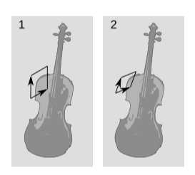
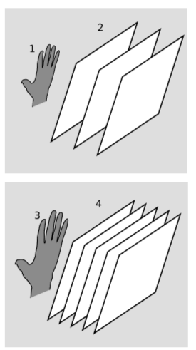
We’ve been visualizing covectors in \(n\) dimensions as stacks of \((n-1)\)-dimensional planes (figure 6.3.1; figure 6.6.1). The volume three-vector should therefore be visualized as a stack of \(3\)-planes in a four-dimensional space. Since most of us can’t visualize things very well in four dimensions, figure \(\PageIndex{8}\) omits one of the dimensions, so that the \(3\)-surfaces appear as two-dimensional planes. The small hand figure \(\PageIndex{1}\) (1) has a certain \(3\)-volume, and the covector that measures it is represented by the stack of \(3\)-planes parallel to it, figure \(\PageIndex{1}\) (2). The bigger hand figure \(\PageIndex{1}\) (3) has twice the \(3\)-volume, and its covector is represented by a stack of planes with half the spacing.

If we step down from four dimensions to three, then the volume covector formed by vectors \(u\) and \(v\) becomes the vector cross product \(S = u×v\), i.e., \(S_k = \epsilon _{ijk} u^i v^j\).

Example \(\PageIndex{7}\): A vector cross product

Consider Euclidean 3-space in Cartesian coordinates. We know from freshman physics that

\[\hat{z} = \hat{x}\times \hat{y}\]

Reexpressing this in the notation above, we have \(u^x = 1\), \(v^y = 1\), and zero for all the other components of \(u\) and \(v\). Since the Levi-Civita tensor vanishes if we have any duplicated indices, its only nonvanishing component that can be relevant here is \(\epsilon _{xyz}= 1\). (Here we assume the standard right-handed orientation for Cartesian coordinates, and we make use of the fact that \(g = diag(1,1,1)\), so that \(detg = 1\).) The result is

\[S_z = \epsilon _{xyz}u^x v^x = 1\]

as expected. (It doesn’t matter here whether we talk about \(S_z\) or \(S^z\), because with this metric, raising and lowering indices doesn’t change the components of a vector.)

Classification of 3-surfaces

A useful application of the \(3\)-volume covector is in classifying \(3\)-surfaces by how they relate to the light cone. If I nail together three sticks, all at right angles to one another, then I can consider them as a set of basis vectors spanning a three-dimensional space of events. This three-space is flat, so we can call it a hyperplane — or just a plane if, as throughout this section, there is no danger of forgetting that it has three dimensions rather than two. All of the events in this plane are simultaneous in my frame of reference. None of these facts depends on the use of right angles; we just need to make sure that the sticks don’t all lie in the same plane.

The business of a physicist is ultimately to make predictions. That is, if given a set of initial conditions, we can say how our system will evolve through time. These initial conditions are in principle measured throughout all of space, and a plane of simultaneity would be a natural choice for the set of points at which to take the measurements. A surface used for this purpose is called a Cauchy surface.

If a plane is a surface of simultaneity according to some observer, then we call it spacelike. Any particle’s world-line must intersect such a plane exactly once, and this is why it works as a Cauchy surface: we are guaranteed to detect the particle, so that we can account for its effect on the evolution of the cosmos. We could take a spacelike plane and reorient it. For a small enough change in the orientation (that is, a change that could be described by small enough changes in the basis vectors), it will remain spacelike.

When a plane is not spacelike, and remains so under any sufficiently small change in orientation, we call it timelike. In Minkowski coordinates, an example would be the \(t-x-y\) plane. A given particle’s world-line might never cross such a surface, and therefore a timelike plane cannot be used as a Cauchy surface.

A plane that is neither spacelike nor timelike is called lightlike. An example is the surface defined by the equation \(x = t\) in Minkowski coordinates.

The above classification can be stated very succinctly by using the \(3\)-volume covector defined in above. A plane is spacelike, lightlike, or timelike, respectively, if the regions it contains are described by \(3\)-volume covectors that are timelike, lightlike, or spacelike. A surface that is smooth but not necessarily flat can be be described locally according to these categories by considering its tangent plane. For example, a light cone is lightlike at each of its points, and since it is lightlike everywhere, we call it a lightlike surface. The event horizon of a black hole is also a lightlike surface. Any spacelike surface, whether curved or flat, can be used as a Cauchy surface.

Lightlike surfaces have some funny properties. Using birdtracks notation, suppose that we form such a surface as the space spanned by the three basis vectors \(\to a\), \(\to b\), and \(\to c\), and let \(S \to \) be the corresponding \(3\)-volume covector. The surface is lightlike, so

\[S \to S = 0\]

Because \(S \to \) is defined as the function giving the \(4\)-volume of a parallelepiped spanned by the bases with a fourth vector \(\to d\), and because this volume vanishes when \(\to d\) is tangent to the surface ( property V2), we have,

\[S \to a = S \to b = S \to c = 0\]

So in this sense \(S \to \) is perpendicular to the surface. In Euclidean space we are used to describing the orientation of a surface in terms of the unit normal vector, and this is very nearly what \(S \to \) is, except that it’s a covector rather than a vector, and it also can’t be made to have unit length, since its magnitude is zero. We could fix the first of these two problems by constructing the vector \(\to S\) that is dual to \(S\to \), but this has a disconcerting effect. Combining \(\PageIndex{17}\) with the definition of \(S\to \), we find that \(\to S\) spans a vanishing \(4\)-volume with the basis vectors, and therefore by V2 we find that \(\to S\) is tangent to the surface. Thus in some sense we have a vector that is both parallel to and tangent to a surface — which avoids being absurd because we are really referring to two different objects, the covector \(S\to \) and the vector \(\to S\).