18.2: Thermal Conductivity

18.2.1 Solid Good Conductors (Metals)

The difference between the thermal conductivities of metals and non-metals is so large that different experimental approaches are needed for the two classes of solids, and in this subsection we deal with metals.

I remember as long ago as when I was in high school one of the experiments we had to do was to measure the conductivity of a metal rod, which, as far as I remember, was about a foot (30 cm) long and maybe two centimetres in diameter. The experiment was called Searle's Rod, or Searle's Bar, after an experimenter in the early years of the twentieth century. The experiment was simple in principle, but very difficult in practice to do accurately, and we were always advised to avoid doing heat experiments in our matriculation examinations. Heat was supplied by an electrical coil wrapped around one end the rod, and the rate of supply of heat was determined from the current through the wire and the potential difference across it, measured with an ammeter and voltmeter respectively. Heat was collected at the other end of the rod by means of a stream of water flowing through a helical tube wrapped around that end of the rod. Thermometers at the beginning and end of this helical tube measured the rise in temperature of the water. Hence one could determine the rate of flow of heat out of the cool end of the rod. If no heat were lost from side of the rod, the rate of flow of heat into the rod (determined electrically) should equal the rate of flow out of it (measured by the rise in temperature of the stream of water through the helical tube). The difference between the two would be a measure of how much heat was lost from the side of the rod. The rod was supposedly well lagged with cotton wool to keep the heat loss small. (I am talking of a high-school experiment here. One could improve on this in a more advanced laboratory by having the rod in a vacuum – so there is no loss of heat by conduction or convection, and highly polished to reduce heat loss by radiation). The temperature gradient along the length of the tube was determined by drilling pits at two points along the rod, filling these with mercury (for good thermal contact), and sticking mercury-in-glass thermometers into these little pools of mercury. One can easily imagine how difficult such an experiment was! At any rate, there was by then enough information to determine the thermal conductivity, for one knew the temperature gradient, from the thermometers stuck into the little mercury pools, and one knew the rate of flow of heat into and out of the rod, and of course one knew the cross-sectional area of the rood. In a more advanced laboratory today, rather than sticking mercury-in-glass thermometers into two mercuryfilled holes, one could measure the temperature at several points along the length of the rod by means of thermocouples or thermistors welded into the rod. If there were no heat losses along the length of the rod, the temperature gradient would be uniform along the rod. In practice, the thermistors would show a nonuniform temperature gradient, and from this one could calculate and allow for the heat loss along the rod. Likewise the temperatures at the inflow and outflow ends of the little helical tube could be measured with some tiny modern device, and all of these electrical connections today would be connected to a computer, which would immediately do all the necessary calculations, including correction of heat loss, and the thermal conductivity would be instantly displayed!

Lees developed the details of the equipment so that much smaller specimens could be used – e.g. a rod just a few cm in length and a few mm in diameter – so that he could enclose it in a Dewar flask and make measurements down to the temperature of liquid air. Three small coils of varnished copper wire were wound round the rod. (By varnished copper wire I mean copper wire whose surface was painted with a layer of varnish of sufficient thickness to insulate the coils electrically but sufficiently thin that good thermal contact with the rod was made.) One of these coils was wound round the upper end of the rod, and supplied heat at that end. The other two coils could be slid up and down to any desired positions on the rod, and they served as resistance thermometers. That is, the local temperature of the rod could be measured by measuring the resistance if the coils. This set-up provided in principle what was necessary to determine the thermal conductivity of the rod, for the rate of input of heat to the rod was determined by the current in the uppermost coil, and the temperature gradient down the rod was measured with the two movable thermometer coils.

An interesting method that has been used (using a rod of roughly the same dimensions as in Searle's Rod experiment – that is to say, about a foot (30 cm) long and one or two cm in diameter − is to pass an electrical current along length of the rod, thus heating it. However, the two ends of the rod are kept at the same temperature (T₁) by keeping them in constant-temperature baths. The temperature of the rod is greatest (T₂) at its mid-point. It can be shown, by a solution of the heat conduction equation, that

\[\sigma_{\text { therm }}=\frac{V^{2}}{8\left(T_{2}-T_{1}\right)} \sigma_{\text { elect }}.\]

Here, V is the electrical potential difference, in volts, across the ends of the rod, σ_therm is the thermal conductivity in W m⁻¹ K⁻¹, and σ_elect is the electrical conductivity, in S m−1 . I haven't derived that equation here (if I can, I may do so later!), but at least you can (I hope!) show that it is dimensionally correct. This method has been used to measure the ratio of the thermal to the electrical conductivity down to temperatures of a few kelvin, as well as at high temperatures.

18.2.2 Solid Poor Conductors (Non-metals)

The most obvious modification that has to be made for the measurement of the thermal conductivity of a poor conductor is in the shape of the sample to be measured. Instead of a long, thin rod, one needs a thin disc. In Lees' Discs experiment, the disc-shaped sample is clamped between two copper discs, one of which is heated with an electrical coil. The temperatures of the two copper discs are measured with thermocouples. This gives enough information, in principle, for the determination of the thermal conductivity, but, as in all thermal experiments, there are numerous refinements both for minimizing heat losses, and for allowing for what heat losses remain.

18.2.3 Liquids and Gases

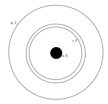
Several methods have been used. Here I mention one straightforward method that has been used for both liquids and gases (i.e. fluids). The fluid is held in a long cylinder of radius b. A wire, of radius a, down the axis of the cylinder is heated electrically. The temperature T₂ of the wire can be measured by measuring its resistance, and the temperature T₁ the wall of the cylinder can be measured with a thermocouple. The rate of flow of heat \( \dot{Q}\) through the fluid is equal to the rate at which electrical energy is supplied to the wire - I²R. Anyone who has been able to work out the electric field between two coaxial cylinders in an elementary electricity course (see the Electricity and Magnetism section of these Notes) will be able to work out the relevant equations, but here goes, anyway.

Consider an elemental cylindrical shell, radii r, r + dr. Its area is 2πrl, where l is the length of the cylinder. If the temperature gradient there is dT/dr (which is negative), the rate of flow of heat, \( \dot{Q}\) (which is known, as explained above) is given by

\[\dot{Q}=-2 \pi r l \sigma \frac{d T}{d r}.\]

Integrate this from r = a, T = T₂ to r = b, T = T₁, and we get

\[\sigma=\frac{\dot{Q}}{2 \pi l\left(T_{2}-T_{1}\right)} \ln \left(\frac{b}{a}\right).\]

This assumes a very long cylinder, and ignores end effects. End effects can be kept small by using a long, thin tube, and can be allowed for by experimenting with tubes of several lengths.