3.9: Thermodynamics Applied to Phase Transitions

At phase coexistence between, say, gas and liquid

\[ \mu_{G}(p, T)=\mu_{L}(p, T).\]

The Clausius-Clapeyron equation relates the slope of a phase coexistence line p_x(T) with the volume and entropy changes when the sample crosses that line:

\[ \frac{d p_{x}}{d T}=\frac{\Delta S}{\Delta V}.\]

Problems

3.37 Thermodynamics applied to the triple point

A triple point has the usual arrangement of a rising gas-solid coexistence line splitting into two rising coexistence lines: a liquid-solid line and a gas-liquid line.

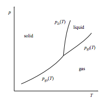
a. Relate the slopes of the three coexistence lines that meet at the triple point to the entropy changes ∆S_gl = S_gas − S_liquid and ∆S_ls = S_liquid − S_solid.

b. Show that the gas-solid coexistence line, when extended beyond the triple point, must extend into the liquid phase as show below left. It must not extend into the gas phase as shown below right.

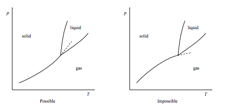
[This result is called “the Schreinemakers 180^o rule” after Franciscus A. H. Schreinemakers, Dutch chemist, 1864–1945.]

c. Show that in most cases, at the triple point the gas-solid coexistence line has nearly the same slope as the gas-liquid coexistence line.

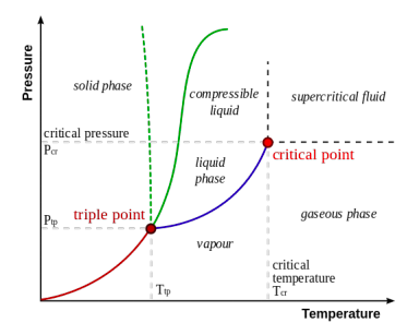
d. The diagram below illustrates the Wikipedia article “Triple point” (15 December 2014). The caption is “A typical phase diagram. The solid green line applies to most substances; the dotted green line gives the anomalous behaviour of water.” Critique this diagram.

3.38 Magnetic phase transitions

The phase diagrams for magnetic systems are usually plotted with temperature on the vertical axis and magnetic field H on the horizontal axis. Show that if such a diagram displays two-phase coexistence along the line T_x(H), then that phase boundary has slope

\[ \frac{d T_{x}}{d H}=-\frac{\Delta M}{\Delta S}\]

where ∆M is the magnetization change accompanying the phase transition.

3.39 Curvature of phase coexistence lines

a. Define

\[ \beta^{\prime}=\frac{\partial v}{\partial T} )_{p}=v \beta \quad \text { and } \quad \kappa_{T}^{\prime}=-\frac{\partial v}{\partial p} )_{T}=v \kappa_{T}\]

and show that, for small changes of temperature δT and pressure δp, the resulting change in chemical potential will be

\[\delta \mu=-s \delta T+v \delta p+\frac{1}{2}\left[-\frac{c_{p}}{T}(\delta T)^{2}+2 \beta^{\prime}(\delta T)(\delta p)-\kappa_{T}^{\prime}(\delta p)^{2}\right]+\cdots .\]

b. Show that for a change along a phase coexistence boundary p_x(T),

\[ \delta p=\frac{d p_{x}}{d T} \delta T+\frac{1}{2} \frac{d^{2} p_{x}}{d T^{2}}(\delta T)^{2}+\cdots .\]

c. If ∆s = s_A − s_B, and similarly for ∆v, ∆c_p, etc., show that for any point on a phase coexistence boundary

\[ 0=-\Delta s \delta T+\Delta v \delta p+\frac{1}{2}\left[-\frac{\Delta c_{p}}{T}(\delta T)^{2}+2 \Delta \beta^{\prime}(\delta T)(\delta p)-\Delta \kappa_{T}^{\prime}(\delta p)^{2}\right]+\cdots .\]

d. Conclude that the slope of the phase coexistence curve is

\[ \frac{d p_{x}}{d T}=\frac{\Delta s}{\Delta v},\]

the usual Clausius-Clapeyron equation, while the second derivative is

\[ \frac{d^{2} p_{x}}{d T^{2}}=\frac{\Delta c_{p}}{T \Delta v}-2 \frac{\Delta \beta^{\prime} \Delta s}{(\Delta v)^{2}}+\frac{\Delta \kappa_{T}^{\prime}(\Delta s)^{2}}{(\Delta v)^{3}},\]

the “second-order Clausius-Clapeyron equation”.