
6.7: Distribution of Speeds


- Last updated
- Sep 10, 2020
- Save as PDF

( \newcommand{\kernel}{\mathrm{null}\,}\)
I am tempted to start by saying "Let f(u)du be the fraction of molecules of which the x-component of their velocities is between u and u + du." But we can go a little further than this with the realization that this distribution must be symmetric about u = 0, and therefore, whatever the function is, it must contain only even powers of u. So we can start with:
Let f(u2)du be the fraction of molecules of which the x-component of their velocities is between u and u + du. Then, unless there is a systematic flow on the x-direction or the x-direction is somehow special, the fraction of molecules with y velocity components between v and v + dv is f(v2)dv, and the fraction of molecules with z velocity components between w and w + dw is f(w2)dw. The fraction of molecules in a box du dv dw of velocity space is f(u2)f(v2)f(w2)du dv dw. Since the distribution of velocity components is independent of direction, this product must be of the form
f(u2)f(v2)f(w2)=F(c2)
or
f(u2)f(v2)f(w2)=F(u2+v2+w2)
(Question: Dimensions of f? Of F?)
It is easy to see that this is satisfied by
f(u2)=Ae±u2/c2n,
where A and cm are constants to be determined. It should also be clear that, of the two possible solutions represented by equation 6.7.3, we must choose the one with the minus sign.
Since we must have
∫∞−∞f(u2)du=1
it follows that
A=1cm√π.
(To see this, you have to know that ∫∞0e−ax2dx=12√πa.)
Thus we now have
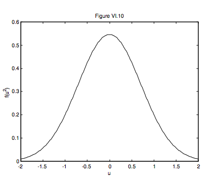
f(u2)=1cm√πe−u2/c2m
This is the gaussian distribution of a velocity component. We shall shortly find a physical interpretation for the constant cm.
The area under the curve represented by equation 6.7.9 is, of course, unity; the maximum value of ( is) /(1 ). 2 f u cm π
Figure VI.10 illustrates this distribution. In this figure, the unit of speed is cm. The area under the curve is 1. The maximum (at u = 0) is 1/√π=0.564. Exercise: Show that the FWHM (full width at half maximum) is 2√ln2cm=1.665cm. This gives one physical interpretation of cm; we shall soon give another one, which will explain the use of m as a subscript.
The gaussian distribution deals with velocity components. We deal now with speeds. The fraction of molecules having speeds between c and c + dc is F(c2) times the volume of a spherical shell in velocity space of radii c and c + dc. (Some readers may recall a similar argument in the Schrödinger equation for the hydrogen atom, in which the probability of the electron's being at a distance between r and r + dr is the probability density ψψ* times the volume of a spherical shell.
You'll notice that physics becomes easier and easier, because you have seen it all before in different contexts. In the present context, F is akin to the ψψ* of wave mechanics, and it could be considered to be a "speed density".) Thus the fraction of molecules having speeds between c and c + dc is
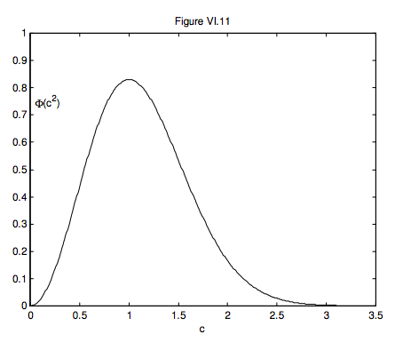
Φ(c2)dc=4c2c3m√πe−c2/c2mdc
I shall leave it to those who are skilled at calculus to show that ∫∞0Φ(c2)dc=1, and also to show that the maximum of this distribution occurs for a speed of c = cm and that the maximum value of Φ (c2) is 4/(cme√π). This provides another interpretation of the constant cm. The speed at which the maximum of the distribution occurs is called the mode of the distribution, or the modal speed – hence the subscript m. Equation 6.7.10 is the Maxwell-Boltzmann distribution of speeds. It is shown in figure VI.7, in which the unit of speed is cm. The area is 1, and the maximum is 4/(e√π)=0.830.
The mean speed ¯c is found from ∫∞0cΦ(c2)dc and the root mean square speed cRMS is found from c2RMS=∫∞0c2Φ(c2)dc. If you have not encountered integrals of this type before, you may find that the first of them is easier than the second. If you can do these integrals, you will find that
¯c=2√πcm and cRMS=√32cm
The root mean square (RMS) speed, for which I am here using the symbol cRMS, is of course the square root of ¯c2. We have seen from Section 6.5 that the mean kinetic energy per molecule, 12m¯c2, is equal to 32kT, so now let's bring it all together:
cm=√π2¯c=0.886¯c=√23cRMS=0.816cRMS=√2kTm=1.414√kTm
¯c=2√πcm=1.128cm=√83πcRMS=0.921cRMS=√8kTπm=1.596√kTm
cRMS=√32cm=1.225cm=√3π8¯c=1.085¯c=√3kTm=1.732√kTm
Gauss:
f(u2)=√m2πkTe−mu22kT.
Maxwell-Boltzmann:
Φ(c2)=√2π(mkT)3/2c2e−mc22kT.
One last thing occurs to me before we leave this section. Can we calculate the median speed c1/2 of the Maxwell-Boltzmann distribution? This is the speed such that half of the molecules are moving slower than c1/2, and half are moving faster. It is the speed that divides the area under the curve in half. If we express speeds in units of cm, we have to find c1/2 such that
4√π∫c1/20c2e−c2dc=12,
or
∫c1/20c2e−c2dc=√π8=0.2215567314
That should keep your computer busy for a while. Mine made the answer c1/2 = 1.087 65 cm.