8.6: The Slopes of Isotherms and Adiabats

For an ideal gas in an isothermal process, PV = constant.

In a reversible adiabatic process:

PV^γ = constant,

TV^γ − 1 = constant,

P^{1 − γ}T^γ = constant.

From these it is easy to see that the ratios of the adiabatic, isothermal, isobaric and isochoric slopes are as follows:

\[ \left(\frac{\partial P}{\partial V}\right)_{S}=\gamma\left(\frac{\partial P}{\partial V}\right)_{T} ; \qquad\left(\frac{\partial V}{\partial T}\right)_{S}=-\frac{1}{\gamma-1}\left(\frac{\partial V}{\partial T}\right)_{P} ; \qquad\left(\frac{\partial P}{\partial T}\right)_{S}=\frac{\gamma}{\gamma-1}\left(\frac{\partial P}{\partial T}\right)_{V}.\]

For example: - isothermal: PV = constant. Take logarithms and differentiate: \(\frac{d P}{P}+\frac{d V}{V}=0\). Hence \( \left(\frac{\partial P}{\partial V}\right)_{T}=-\frac{P}{V}\). adiabatic: PV^γ = constant. Take logarithms and differentiate: \( \frac{d P}{P}+\gamma \frac{d V}{V}=0\). Hence \( \left(\frac{\partial P}{\partial V}\right)_{S}=-\gamma \frac{P}{V}\). The other two relations can be obtained in a similar manner.

Do these relations hold in general for any equation of state, or are they valid only for an ideal gas? In this section, we shall see that they are valid in general for any equation of state, and are not restricted to the equation of state for an ideal gas.

Let us imagine that the state of the working substance (be it gas, liquid or solid) starts in PVT space at point A (P, V, T_A). We are going to take it to a new point B (P + δP, V + δV, T_B). As I have drawn it in Figure VIII.3, δP is positive, δV is negative, and T_B > T_A.

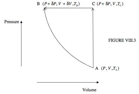
We first suppose that we make this move by a single, adiabatic process. In that case no heat is added to or lost from the system, and the increase in the internal energy is −PδV.

Alternatively, B can be reached in two stages:

An isochoric path from A to a new point C (P + δP, V, T_C), followed by

An isobaric path from C to B.

As I have drawn it in Figure VIII.3, T_C > T_B > T_A .

In the isochoric process, no work is done by or on the system, and the increase in the internal energy is equal to the heat added to the system, C_V (T_C − T_A).

In the isobaric process, the increase in the internal energy is equal to the work done on the system, −PδV, minus the heat lost from the system, C_P (T_C − T_B); that is, −C_P (T_C − T_B) − PδV.

Therefore, since the total increase in internal energy is route-independent,

\[ -P \delta V=C_{V}\left(T_{\mathrm{c}}-T_{\mathrm{A}}\right)-C_{P}\left(T_{\mathrm{C}}-T_{\mathrm{B}}\right)-P \delta V.\]

Cancel PδV and write γ for C_P/C_V, so that

\[ \left(T_{\mathrm{C}}-T_{\mathrm{A}}\right)=\gamma\left(T_{\mathrm{C}}-T_{\mathrm{B}}\right).\]

But \( T_{\mathrm{C}}=T_{\mathrm{A}}+\left(\frac{\partial T}{\partial P}\right)_{V} \delta P\) and \( T_{\mathrm{B}}=T_{\mathrm{C}}+\left(\frac{\partial T}{\partial V}\right)_{P} \delta V\).

[Reminder: Here δP means P_C − P_A (which, in the way in which I have drawn it in figure VIII.3, is positive) and δV means V_B − V_C (which, in the way in which I have drawn it in figure VIII.3, is negative).]

Therefore

\[ \left(\frac{\partial T}{\partial P}\right)_{V} \delta P=-\gamma\left(\frac{\partial T}{\partial V}\right)_{P} \delta V.\]

Divide both sides by δV and go to the infinitesimal limit, recalling that δP and δV are related through an adiabatic path:

\[ \left(\frac{\partial T}{\partial P}\right)_{V}\left(\frac{\partial P}{\partial V}\right)_{S}=-\gamma\left(\frac{\partial T}{\partial V}\right)_{P}.\]

Therefore

\[ \left(\frac{\partial P}{\partial V}\right)_{S}=-\gamma\left(\frac{\partial T}{\partial V}\right)_{P}\left(\frac{\partial P}{\partial T}\right)_{V}.\]

But \( \left(\frac{\partial T}{\partial V}\right)_{P}\left(\frac{\partial P}{\partial T}\right)_{V}\left(\frac{\partial V}{\partial P}\right)_{T}=-1\), so \( \left(\frac{\partial T}{\partial V}\right)_{P}\left(\frac{\partial P}{\partial T}\right)_{V}=-\left(\frac{\partial P}{\partial V}\right)_{T}\).

Therefore

\[ \left(\frac{\partial P}{\partial V}\right)_{S}=\gamma\left(\frac{\partial P}{\partial V}\right)_{T}.\]

Thus, as for the ideal gas, the slope of the adiabat is γ times the slope of the isotherm, only this time we have made no assumption about the equation of state.

The other two relations (equations 8.6.1 b,c) can be dealt with as follows.

Equation 8.6.3 can be rearranged to read

\[ T_{\mathrm{B}}-T_{\mathrm{A}}=-(\gamma-1)\left(T_{\mathrm{B}}-T_{\mathrm{C}}\right)\]

But \( T_{\mathrm{B}}=T_{\mathrm{A}}+\left(\frac{\partial T}{\partial V}\right)_{S} \delta V\) and \( T_{\mathrm{B}}=T_{\mathrm{C}}+\left(\frac{\partial T}{\partial V}\right)_{P} \delta V\).

Hence

\[ \left(\frac{\partial V}{\partial T}\right)_{S}=-\frac{1}{\gamma-1}\left(\frac{\partial V}{\partial T}\right)_{P}, \]

which is the same as equation 8.6.1 b, but without any assumption about the equation of state.

Note also that

\[ \left(\frac{\partial P}{\partial V}\right)_{T}\left(\frac{\partial V}{\partial T}\right)_{P}\left(\frac{\partial T}{\partial P}\right)_{V}=-1.\]

Combine this with equations 8.6.7 and 8.6.9 to obtain

\[ \frac{1}{\gamma}\left(\frac{\partial P}{\partial V}\right)_{S}(\gamma-1)\left(\frac{\partial V}{\partial T}\right)_{S}\left(\frac{\partial T}{\partial P}\right)_{V}=1.\]

Therefore

\[ \left(\frac{\partial P}{\partial T}\right)_{V}=\frac{\gamma-1}{\gamma}\left(\frac{\partial P}{\partial V}\right)_{S}\left(\frac{\partial V}{\partial T}\right)_{S}=\frac{\gamma-1}{\gamma}\left(\frac{\partial P}{\partial T}\right)_{S}.\]

Therefore

\[ \left(\frac{\partial P}{\partial T}\right)_{S}=\frac{\gamma}{\gamma-1}\left(\frac{\partial P}{\partial T}\right)_{V},\]

which is the same as equation 8.6.1 c, but without any assumption about the equation of state.