2.2: Microcanonical ensemble and distribution

Figure \(\PageIndex{1}\): A very schematic image of the microcanonical ensemble. (Actually, the ensemble deals with quantum states rather than energy levels. An energy level may be degenerate, i.e. correspond to several states.)

This ensemble serves as the basis for the formulation of the postulate which is most frequently called the microcanonical distribution (or, more adequately, “the main statistical postulate” or “the main statistical hypothesis”): in the thermodynamic equilibrium of a microcanonical ensemble, all its states have equal probabilities,

Microcanonical distribution:

\[\boxed{ W_m = \frac{1}{M} = \text{const.}} \label{20}\]

Though in some constructs of statistical mechanics this equality is derived from other axioms, which look more plausible to their authors, I believe that Equation (\ref{20}) may be taken as the starting point of the statistical physics, supported “just” by the compliance of all its corollaries with experimental observations.

Note that the postulate (\ref{20}) is closely related to the macroscopic irreversibility of the systems that are microscopically virtually reversible (closed): if such a system was initially in a certain state, its time evolution with just minuscule interactions with the environment (which is necessary for reaching the thermodynamic equilibrium) eventually leads to the uniform distribution of its probability among all states with essentially the same energy. Each of these states is not “better” than the initial one; rather, in a macroscopic system, there are just so many of these states that the chance to find the system in the initial state is practically nil – again, think about the ink drop diffusion into a glass of water.⁹

Now let us find a suitable definition of the entropy \(S\) of a microcanonical ensemble’s member – for now, in the thermodynamic equilibrium only. This was done in 1877 by another giant of statistical physics, Ludwig Eduard Boltzmann – on the basis of the prior work by James Clerk Maxwell on the kinetic theory of gases – see Sec. 3.1 below. In the present-day terminology, since \(S\) is a measure of disorder, it should be related to the amount of information¹⁰ lost when the system went irreversibly from the full order to the full disorder, i.e. from one definite state to the microcanonical distribution (\ref{20}). In an even more convenient formulation, this is the amount of information necessary to find the exact state of your system in a microcanonical ensemble.

In the information theory, the amount of information necessary to make a definite choice between two options with equal probabilities (Figure \(\PageIndex{2a}\)) is defined as

\[I (2) \equiv \log_2 2 = 1 \label{21}\]

This unit of information is called a bit.

Figure \(\PageIndex{2}\): “Logarithmic trees” of binary decisions for choosing between (a) \(M = 2\), and (b) \(M = 4\) opportunities with equal probabilities.

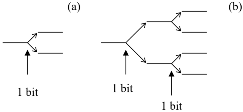
Now, if we need to make a choice between four equally probable opportunities, it can be made in two similar steps (Figure \(\PageIndex{2b}\)), each requiring one bit of information, so that the total amount of information necessary for the choice is

\[I (4) = 2 I (2) = 2 \equiv \log_2 4. \label{22}\]

An obvious extension of this process to the choice between \(M = 2^m\) states gives

\[I (M) = mI (2) = m \equiv \log_2 M \label{23}\]

\[ S \equiv \ln M. \label{24a}\]

Using Equation (\ref{20}), we may recast this definition in its most frequently used form

Entropy in equilibrium:

\[\boxed{ S = \ln \frac{1}{W_m} = -\ln W_m.} \label{24b}\]

(Again, please note that Equation (\ref{24a} - \ref{24b}) is valid in thermodynamic equilibrium only!)

Note that Equation (\ref{24a} - \ref{24b}) satisfies the major properties of the entropy discussed in thermodynamics. First, it is a unique characteristic of the disorder. Indeed, according to Equation (\ref{20}), \(M\) (at fixed \(\Delta E\)) is the only possible measure characterizing the microcanonical distribution, and so is its unique function \(\ln M\). This function also satisfies another thermodynamic requirement to the entropy, of being an extensive variable. Indeed, for several independent systems, the joint probability of a certain state is just a product of the partial probabilities, and hence, according to Equation (\ref{24a} - \ref{24b}), their entropies just add up.

Now let us see whether Eqs. (\ref{20}) and (\ref{24a} - \ref{24b}) are compatible with the \(2^{nd}\) law of thermodynamics. For that, we need to generalize Equation (\ref{24a} - \ref{24b}) for \(S\) to an arbitrary state of the system (generally, out of thermodynamic equilibrium), with an arbitrary set of state probabilities \(W_m\). Let us first recognize that \(M\) in Equation (\ref{24a} - \ref{24b}) is just the number of possible ways to commit a particular system to a certain state \(m\) \((m = 1, 2,...M)\), in a statistical ensemble where each state is equally probable. Now let us consider a more general ensemble, still consisting of a large number \(N >> 1\) of similar systems, but with a certain number \(N_m = W_mN >> 1\) of systems in each of \(M\) states, with the factors \(W_m\) not necessarily equal. In this case, the evident generalization of Equation (\ref{24a} - \ref{24b}) is that the entropy \(S_N\) of the whole ensemble is

\[S_N \equiv \ln M (N_1, N_2 , ...), \label{25}\]

where \(M (N_1, N_2,...)\) is the number of ways to commit a particular system to a certain state \(m\) while keeping all numbers \(N_m\) fixed. This number \(M (N_1, N_2,...)\) is clearly equal to the number of ways to distribute \(N\) distinct balls between \(M\) different boxes, with the fixed number \(N_m\) of balls in each box, but in no particular order within it. Comparing this description with the definition of the so-called multinomial coefficients,¹² we get

\[ M\left(N_{1}, N_{2}, \ldots\right)={ }^{N} C_{N_{1}, N_{2}, \ldots, N_{M}} \equiv \frac{N !}{N_{1} ! N_{2} ! \ldots N_{M} !}, \quad \text { with } N=\sum_{m=1}^{M} N_{m} \label{26}\]

To simplify the resulting expression for \(S_N\), we can use the famous Stirling formula, in its crudest, de Moivre’s form,¹³ whose accuracy is suitable for most purposes of statistical physics:

\[ \ln (N!)_{N\rightarrow\infty} \rightarrow N(\ln N-1). \label{27}\]

When applied to our current problem, this formula gives the following average entropy per system,¹⁴

\[ \begin{align} S & \equiv \frac{S_{N}}{N}=\frac{1}{N}\left[\ln (N !)-\sum_{m=1}^{M} \ln \left(N_{m} !\right)\right]_{N_{m} \rightarrow \infty} \rightarrow \frac{1}{N}\left[N(\ln N-1)-\sum_{m=1}^{M} N_{m}\left(\ln N_{m}-1\right)\right] \nonumber\\ & \equiv-\sum_{m=1}^{M} \frac{N_{m}}{N} \ln \frac{N_{m}}{N} \end{align} \label{28}\]

and since this result is only valid in the limit \(N_m \rightarrow \infty\) anyway, we may use Equation (\(2.1.2\)) to represent it as

Entropy out of equilibrium:

\[ \boxed{ S = -\sum^M_{m = 1} W_m \ln W_m = \sum^M_{m=1} W_m \ln \frac{1}{W_m}. } \label{29}\]

Now let us find what distribution of probabilities \(W_m\) provides the largest value of the entropy (\ref{29}). The answer is almost evident from a good glance at Equation (\ref{29}). For example, if for a subgroup of \(M’ \leq M\) states the coefficients \(W_m\) are constant and equal to \(1/M’\), so that \(W_m = 0\) for all other states, all \(M’\) non-zero terms in the sum (\ref{29}) are equal to each other, so that

\[S = M' \frac{1}{M'} \ln M' \equiv \ln M',\label{30}\]

and the closer \(M’\) to its maximum value \(M\) the larger \(S\). Hence, the maximum of \(S\) is reached at the uniform distribution given by Equation (\ref{24a} - \ref{24b}).

In order to prove this important fact more strictly, let us find the maximum of the function given by Equation (\ref{29}). If its arguments \(W_1, W_2, ...W_M\) were completely independent, this could be done by finding the point (in the \(M\)-dimensional space of the coefficients \(W_m\)) where all partial derivatives \(\partial S/\partial W_m\) equal zero. However, since the probabilities are constrained by the condition (\(2.1.4\)), the differentiation has to be carried out more carefully, taking into account this interdependence:

\[\left[\frac{\partial}{\partial W_{m}} S\left(W_{1}, W_{2}, \ldots\right)\right]_{\text {cond }}=\frac{\partial S}{\partial W_{m}}+\sum_{m^{\prime} \neq m} \frac{\partial S}{\partial W_{m^{\prime}}} \frac{\partial W_{m^{\prime}}}{\partial W_{m}} . \label{31}\]

At the maximum of the function \(S\), all such expressions should be equal to zero simultaneously. This condition yields \(\partial S/\partial W_m = \lambda \), where the so-called Lagrange multiplier \(\lambda\) is independent of \(m\). Indeed, at such point Equation (\ref{31}) becomes

\[\left[\frac{\partial}{\partial W_{m}} S\left(W_{1}, W_{2}, \ldots\right)\right]_{\text {cond }}=\lambda+\sum_{m^{\prime} \neq m} \lambda \frac{\partial W_{m^{\prime}}}{\partial W_{m}} \equiv \lambda\left(\frac{\partial W_{m}}{\partial W_{m}}+\sum_{m^{\prime} \neq m} \frac{\partial W_{m^{\prime}}}{\partial W_{m}}\right) \equiv \lambda \frac{\partial}{\partial W_{m}}(1)=0 . \label{32}\]

For our particular expression (\ref{29}), the condition \(\partial S/\partial W_m = \lambda\) yields

\[\frac{\partial S}{\partial W_{m}} \equiv \frac{d}{d W_{m}}\left[-W_{m} \ln W_{m}\right] \equiv-\ln W_{m}-1=\lambda . \label{33}\]

The last equality holds for all \(m\) (and hence the entropy reaches its maximum value) only if \(W_m\) is independent on \(m\). Thus the entropy (\ref{29}) indeed reaches its maximum value (\ref{24a} - \ref{24b}) at equilibrium.

To summarize, we see that the statistical definition (\ref{24a} - \ref{24b}) of entropy does fit all the requirements imposed on this variable by thermodynamics. In particular, we have been able to prove the \(2^{nd}\) law of thermodynamics using that definition together with the fundamental postulate (\ref{20}).

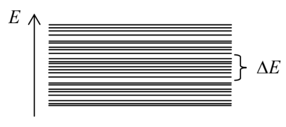
Now let me discuss one possible point of discomfort with that definition: the values of \(M\), and hence \(W_m\), depend on the accepted energy interval \(\Delta E\) of the microcanonical ensemble, for whose choice no exact guidance is offered. However, if the interval \(\Delta E\) contains many states, \(M >> 1\), as was assumed before, then with a very small relative error (vanishing in the limit \(M \rightarrow \infty \)), \(M\) may be represented as

\[ M = g(E)\Delta E, \label{34}\]

where \(g(E)\) is the density of states of the system:

\[g (E) \equiv \frac{d\Sigma (E)}{dE}, \label{35}\]

\(\Sigma (E)\) being the total number of states with energies below \(E\). (Note that the average interval \(\delta E\) between energy levels, mentioned at the beginning of this section, is just \(\Delta E/M = 1/g(E)\).) Plugging Equation (\ref{34}) into Equation (\ref{24a} - \ref{24b}), we get

\[ S = \ln M = \ln g(E) + \ln \Delta E, \label{36}\]

so that the only effect of a particular choice of \(\Delta E\) is an offset of the entropy by a constant, and in Chapter 1 we have seen that such constant shift does not affect any measurable quantity. Of course, Equation (\ref{34}), and hence Equation (\ref{36}) are only precise in the limit when the density of states \(g(E)\) is so large that the range available for the appropriate choice of \(\Delta E\):

\[g^{-1} (E) << \Delta E << E, \label{37}\]

is sufficiently broad: \(g(E)E = E/\delta E >> 1\).

In order to get some feeling of the functions \(g(E)\) and \(S(E)\) and the feasibility of the condition (\ref{37}), and also to see whether the microcanonical distribution may be directly used for calculations of thermodynamic variables in particular systems, let us apply it to a microcanonical ensemble of many sets of \(N >> 1\) independent, similar harmonic oscillators with frequency \(\omega \). (Please note that the requirement of a virtually fixed energy is applied, in this case, to the total energy \(E_N\) of each set of oscillators, rather to energy \(E\) of a single oscillator – which may be virtually arbitrary, though certainly much less than \(E_N \sim NE >> E\).) Basic quantum mechanics tells us¹⁷ that the eigenenergies of such an oscillator form a discrete, equidistant spectrum:

\[E_{m}=\hbar \omega\left(m+\frac{1}{2}\right), \text { where } m=0,1,2, \ldots \label{38}\]

If \(\omega\) is kept constant, the ground-state energy \(\hbar \omega /2\) does not contribute to any thermodynamic properties of the system,¹⁸ so that for the sake of simplicity we may take that point as the energy origin, and replace Equation (\ref{38}) with \(E_m = m\hbar \omega \). Let us carry out an approximate analysis of the system for the case when its average energy per oscillator,

\[E = \frac{E_N}{N}, \label{39}\]

is much larger than the energy quantum \(\hbar \omega \).

For one oscillator, the number of states with energy \(\varepsilon_1\) below a certain value \(E_1 >> \hbar \omega\) is evidently \(\Sigma (E_1) \approx E_1/\hbar \omega \equiv (E_1/\hbar \omega )/1!\) (Figure \(\PageIndex{3a}\)). For two oscillators, all possible values of the total energy \((\varepsilon_1 + \varepsilon_2)\) below some level \(E_2\) correspond to the points of a 2D square grid within the right triangle shown in Figure \(\PageIndex{3b}\), giving \(\Sigma (E_2) \approx (1/2)(E_2/\hbar \omega )^2 \equiv (E_2/\hbar \omega )^{2}/2!\). For three oscillators, the possible values of the total energy \((\varepsilon_1 + \varepsilon_2 + \varepsilon_3)\) correspond to those points of the 3D cubic grid, that fit inside the right pyramid shown in Figure \(\PageIndex{3c}\), giving \(\Sigma (E_3) \approx (1/3)[(1/2)(E_3/\hbar \omega )^3] \equiv (E_3/\hbar \omega )^3/3!\), etc.

Figure \(\PageIndex{3}\): Calculating functions \(\Sigma (E_N)\) for systems of (a) one, (b) two, and (c) three harmonic oscillators.

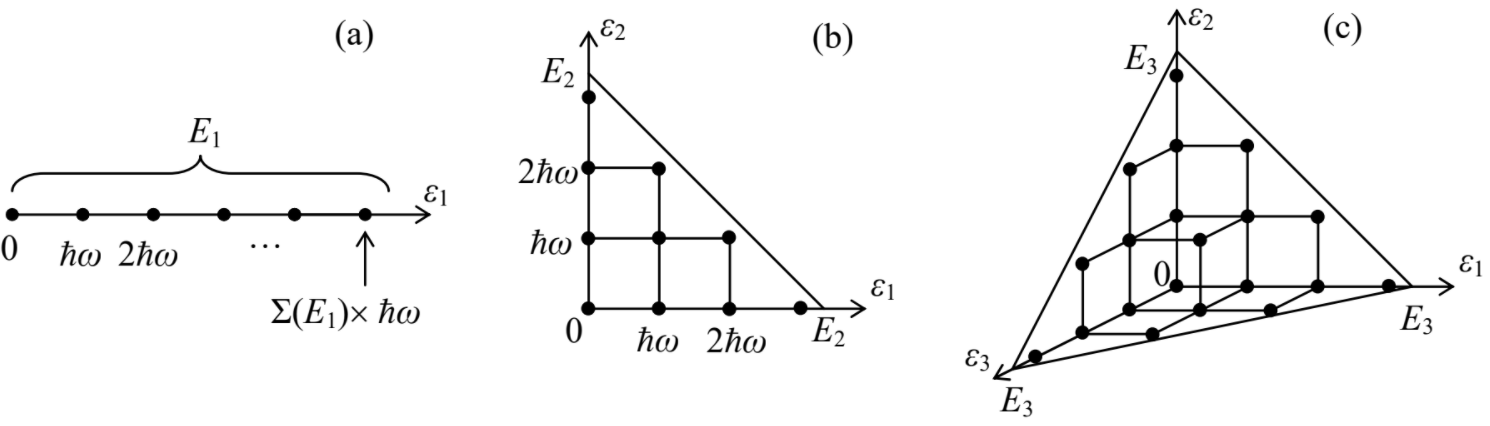
An evident generalization of these formulas to arbitrary \(N\) gives the number of states¹⁹ .

\[\Sigma (E_N) \approx \frac{1}{N!} \left( \frac{E_N}{\hbar \omega}\right)^N. \label{40}\]

Differentiating this expression over the energy, we get

\[g(E_N) \equiv \frac{d\Sigma (E_N)}{dE_N} = \frac{1}{(N-1)!} \frac{E^{N-1}_{N}}{(\hbar \omega)^N}, \label{41}\]

so that

\[S_N (E_N ) = \ln g(E_N ) + \text{ const } = − \ln [(N −1)!]+ (N −1) \ln E_N − N \ln (\hbar \omega ) + \text{ const}. \label{42}\]

For \(N >> 1\) we can ignore the difference between \(N\) and \((N – 1)\) in both instances, and use the Stirling formula (\ref{27}) to simplify this result as

\[S_{N}(E)-\text { const } \approx N\left(\ln \frac{E_{N}}{N \hbar \omega}+1\right) \approx N\left(\ln \frac{E}{\hbar \omega}\right) \equiv \ln \left[\left(\frac{E} {\hbar \omega}\right)^{N}\right] \label{43}\]

(The second, approximate step is only valid at very high \(E/\hbar \omega\) ratios, when the logarithm in Equation (\ref{43}) is substantially larger than 1.) Returning for a second to the density of states, we see that in the limit \(N \rightarrow \infty \), it is exponentially large:

\[g(E_N) = e^{S_N} \approx \left(\frac{E}{\hbar \omega} \right)^N, \label{44}\]

so that the conditions (\ref{37}) may be indeed satisfied within a very broad range of \(\Delta E\).

Now we can use Equation (\ref{43}) to find all thermodynamic properties of the system, though only in the limit \(E >> \hbar \omega \). Indeed, according to thermodynamics, if the system’s volume and the number of particles in it are fixed, the derivative \(dS/dE\) is nothing else than the reciprocal temperature in thermal equilibrium – see Equation (\(1.2.6\)). In our current case, we imply that the harmonic oscillators are distinct, for example by their spatial positions. Hence, even if we can speak of some volume of the system, it is certainly fixed.²⁰ Differentiating Equation (\ref{43}) over energy \(E\), we get

Classical oscillator: average energy

\[\boxed{\frac{1}{T} \equiv \frac{dS_N}{dE_N} = \frac{N}{E_N} = \frac{1}{E}.} \label{45}\]

Reading this result backward, we see that the average energy \(E\) of a harmonic oscillator equals \(T\) (i.e. \(k_BT_K\) is SI units). At this point, the first-time student of thermodynamics should be very much relieved to see that the counter-intuitive thermodynamic definition (\(1.2.6\)) of temperature does indeed correspond to what we all have known about this notion from our kindergarten physics courses.

The result (\ref{45}) may be readily generalized. Indeed, in quantum mechanics, a harmonic oscillator with eigenfrequency \(\omega\) may be described by the Hamiltonian operator

\[\hat{H} = \frac{\hat{p}^2}{2m}+\frac{\kappa \hat{q}^2}{2},\label{46}\]

where \(q\) is some generalized coordinate, \(p\) is the corresponding generalized momentum, \(\mathbf{m}\) is oscillator’s mass,²¹ and \(\kappa\) is the spring constant, so that \(\omega = (\kappa /\mathbf{m})^{1/2}\). Since in the thermodynamic equilibrium the density matrix is always diagonal in the basis of stationary states \(m\) (see Sec. 1 above), the quantum mechanical averages of the kinetic and potential energies may be found from Equation (\(2.1.7\)):

\[\left\langle\frac{p^{2}}{2 \mathbf{m}}\right\rangle=\sum_{m=0}^{\infty} W_{m}\left\langle m\left|\frac{\hat{p}^{2}}{2 \mathbf{m}}\right| m\right\rangle, \quad\left\langle\frac{\kappa q^{2}}{2}\right\rangle=\sum_{m=0}^{\infty} W_{m}\left\langle m\left|\frac{\kappa \hat{q}^{2}}{2}\right| m\right\rangle \label{47}\]

where \(W_m\) is the probability to occupy the \(m^{th}\) energy level, and bra- and ket-vectors describe the stationary state corresponding to that level.²² However, both classical and quantum mechanics teach us that for any \(m\), the bra-ket expressions under the sums in Eqs. (\ref{47}), which represent the average kinetic and mechanical energies of the oscillator on its \(m^{th}\) energy level, are equal to each other, and hence each of them is equal to \(E_m/2\). Hence, even though we do not know the probability distribution \(W_m\) yet (it will be calculated in Sec. 5 below), we may conclude that in the “classical limit” \(T >> \hbar \omega \),

\[\boxed{ \left\langle\frac{p^{2}}{2 \mathbf{m}}\right\rangle= \left\langle\frac{\kappa q^{2}}{2}\right\rangle = \frac{T}{2}.} \label{48}\]

\[\hat{H} = \sum_j \hat{H}_j, \quad \text{with } \hat{H}_j = \frac{\hat{p}^2_j}{2\mathbf{m}_j} + \frac{\kappa_j \hat{q}^2_j}{2}, \label{49}\]

with (generally, different) frequencies \(\omega_j = (\kappa_j/\mathbf{m}_j)^{1/2}\). Since the “modes” (effective harmonic oscillators) contributing to this Hamiltonian, are independent, the result (\ref{48}) is valid for each of the modes. This is the famous equipartition theorem: at thermal equilibrium with \(T >> \hbar \omega_j\), the average energy of each so called half-degree of freedom (which is defined as any variable, either \(p_j\) or \(q_j\), giving a quadratic contribution to the system’s Hamiltonian), is equal to \(T/2\).²⁴ In particular, for each of three Cartesian component contributions to the kinetic energy of a free-moving particle, this theorem is valid for any temperature, because such components may be considered as 1D harmonic oscillators with vanishing potential energy, i.e. \(\omega_j = 0\), so that condition \(T >> \hbar \omega_j\) is fulfilled at any temperature.

I believe that this case study of harmonic oscillator systems was a fair illustration of both the strengths and the weaknesses of the microcanonical ensemble approach.²⁵ On one hand, we could readily calculate virtually everything we wanted in the classical limit \(T >> \hbar \omega \), but calculations for an arbitrary \(T \sim \hbar \omega \), though possible, are rather unpleasant because for that, all vertical steps of the function \(\Sigma (E_N)\) have to be carefully counted. In Sec. 4, we will see that other statistical ensembles are much more convenient for such calculations.

Let me conclude this section with a short notice on deterministic classical systems with just a few degrees of freedom (and even simpler mathematical objects called “maps”) that may exhibit essentially disordered behavior, called the deterministic chaos.²⁶ Such chaotic system may be approximately characterized by an entropy defined similarly to Equation (\ref{29}), where \(W_m\) are the probabilities to find it in different small regions of phase space, at well-separated small time intervals. On the other hand, one can use an expression slightly more general than Equation (\ref{29}) to define the so-called Kolmogorov (or “Kolmogorov-Sinai”) entropy \(K\) that characterizes the speed of loss of the information about the initial state of the system, and hence what is called the “chaos depth”. In the definition of \(K\), the sum over \(m\) is replaced with the summation over all possible permutations \(\{m\} = m_0, m_1, ..., m_{N-1}\) of small space regions, and \(W_m\) is replaced with \(W_{\{m\}}\), the probability of finding the system in the corresponding regions m at time moment \(t_m\), with \(t_m = m\tau \), in the limit \(\tau \rightarrow 0\), with \(N\tau =\) const. For chaos in the simplest objects, 1D maps, \(K\) is equal to the Lyapunov exponent \(\lambda > 0\).²⁷ For systems of higher dimensionality, which are characterized by several Lyapunov exponents \(\lambda \), the Kolmogorov entropy is equal to the phase-space average of the sum of all positive \(\lambda \). These facts provide a much more practicable way of (typically, numerical) calculation of the Kolmogorov entropy than the direct use of its definition.²⁸