2.5: Harmonic Oscillator Statistics

The last property may be immediately used in our first example of the Gibbs distribution application to a particular, but very important system – the harmonic oscillator, for a much more general case than was done in Sec. 2, namely for an arbitrary relation between \(T\) and \(\hbar \omega \).³⁸ Let us consider a canonical ensemble of similar oscillators, each in a contact with a heat bath of temperature \(T\). Selecting the ground-state energy \(\hbar \omega /2\) for the origin of \(E\), the oscillator eigenenergies (\(2.2.28\)) become \(E_m = m\hbar \omega\) (with \(m = 0, 1,…\)), so that the Gibbs distribution (\(2.4.7\)) for probabilities of these states is

\[W_m = \frac{1}{Z} \text{exp}\left\{-\frac{E_m}{T}\right\} = \frac{1}{Z} \text{exp}\left\{-\frac{m \hbar \omega}{T}\right\}, \label{66}\]

with the following statistical sum:

\[ Z = \sum^{\infty}_{m=0} \text{exp}\left\{-\frac{m \hbar \omega}{T}\right\} \equiv \sum^{\infty}_{m=0} \lambda^m, \quad \text{ where } \lambda \equiv \text{exp}\left\{-\frac{\hbar \omega}{T}\right\} \leq 1 \label{67}\]

This is just the well-known infinite geometric progression (the “geometric series”),³⁹ with the sum

Quantum oscillator: statistics

\[\boxed{ Z = \frac{1}{1- \lambda} \equiv \frac{1}{1- e^{ −\hbar \omega/T}},} \label{68}\]

so that Equation (\ref{66}) yields

Quantum oscillator: statistics

\[ \boxed{ W_m = \left( 1 - e^{-\hbar \omega / T}\right) E^{− m \hbar \omega / T}. } \label{69}\]

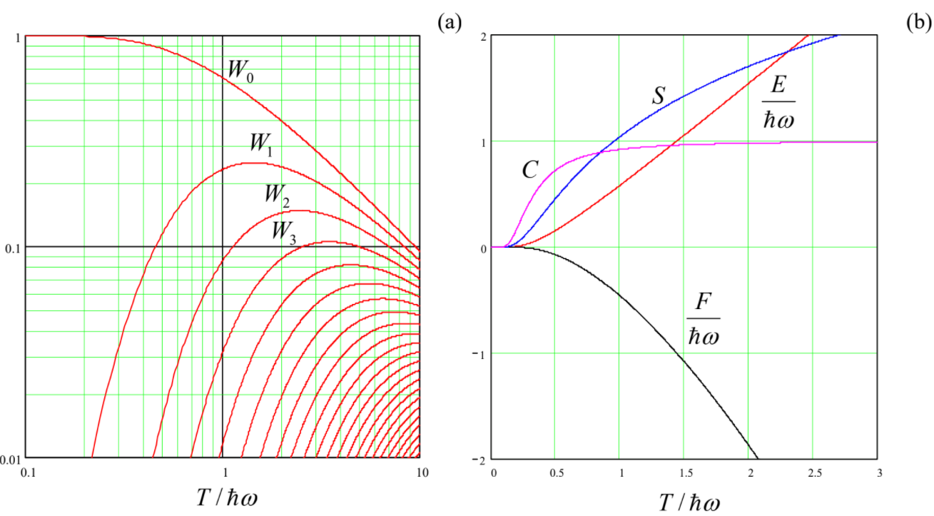
Figure \(\PageIndex{1a}\) shows \(W_m\) for several lower energy levels, as functions of temperature, or rather of the \(T/\hbar \omega\) ratio. The plots show that the probability to find the oscillator in each particular state (except for the ground one, with \(m = 0\)) vanishes in both low- and high-temperature limits, and reaches its maximum value \(W_m \sim 0.3/m\) at \(T \sim m\hbar \omega \), so that the contribution \(m\hbar \omega W_m\) of each excited level to the average oscillator energy \(E\) is always smaller than \(\hbar \omega \).

Figure \(\PageIndex{1}\): Statistical and thermodynamic parameters of a harmonic oscillator, as functions of temperature.

This average energy may be calculated in either of two ways: either using Equation (\(2.4.10\)) directly:

\[ E = \sum^{\infty}_{m=0} E_m W_m = \left( 1 - e^{-\hbar \omega / T}\right) \sum^{\infty}_{m=0} m \hbar \omega e^{-m\hbar \omega / T}, \label{70}\]

or (simpler) using Equation (\(2.4.11\)), as

\[E = - \frac{\partial}{\partial \beta} \ln Z = \frac{\partial}{\partial \beta} \ln (1 - \text{exp}\left\{-\beta \hbar \omega\right\}), \quad \text{ where } \beta \equiv \frac{1}{T}. \label{71}\]

Quantum oscillator: average energy

\[\boxed{E = E(\omega,T) = \hbar \omega \frac{1}{e^{\hbar \omega /T} - 1}, } \label{72}\]

which is valid for arbitrary temperature and plays a key role in many fundamental problems of physics. The red line in Figure \(\PageIndex{1b}\) shows this result as a function of the normalized temperature. At relatively low temperatures, \(T << \hbar \omega \), the oscillator is predominantly in its lowest (ground) state, and its energy (on top of the constant zero-point energy \(\hbar \omega /2\), which was used in our calculation as the reference) is exponentially small: \(E \approx \hbar \omega \text{exp}\{-\hbar \omega /T\} << T, \hbar \omega \). On the other hand, in the high-temperature limit, the energy tends to \(T\). This is exactly the result (a particular case of the equipartition theorem) that was obtained in Sec. 2 from the microcanonical distribution. Please note how much simpler is the calculation using the Gibbs distribution, even for an arbitrary ratio \(T/\hbar \omega \).

To complete the discussion of the thermodynamic properties of the harmonic oscillator, we can calculate its free energy using Equation (\(2.4.13\)):

\[F = T \ln \frac{1}{Z} = T \ln (1 - e^{−\hbar \omega /T} ). \label{73}\]

Now the entropy may be found from thermodynamics: either from the first of Eqs. (\(1.4.12\)), \(S = –(\partial F/\partial T)_V\), or (even more easily) from Equation (\(1.4.10\)): \(S = (E – F)/T\). Both relations give, of course, the same result:

\[S=\frac{\hbar \omega}{T} \frac{1}{e^{\hbar \omega / T}-1}-\ln \left(1-e^{-\hbar \omega / T}\right) .\label{74}\]

Finally, since in the general case the dependence of the oscillator properties (essentially, of \(\omega \)) on volume \(V\) is not specified, such variables as \(P\), \(\mu \), \(G\), \(W\), and \(\Omega\) are not defined, and what remains is to calculate the average heat capacity \(C\) per one oscillator:

\[C=\frac{\partial E}{\partial T}=\left(\frac{\hbar \omega}{T}\right)^{2} \frac{e^{\hbar \omega / T}}{\left(e^{\hbar \omega / T}-1\right)^{2}} \equiv\left[\frac{\hbar \omega / 2 T}{\sinh (\hbar \omega / 2 T)}\right]^{2} .\label{75}\]

The calculated thermodynamic variables are plotted in Figure \(\PageIndex{1b}\). In the low-temperature limit \((T << \hbar \omega )\), they all tend to zero. On the other hand, in the high-temperature limit \((T >> \hbar \omega )\), \(F \rightarrow –T \ln (T/\hbar \omega )\rightarrow –\infty \), \(S \rightarrow \ln (T/\hbar \omega ) \rightarrow +\infty\), and \(C \rightarrow 1\) (in the SI units, \(C \rightarrow k_B\)). Note that the last limit is the direct corollary of the equipartition theorem: each of the two “half-degrees of freedom” of the oscillator gives, in the classical limit, the same contribution \(C = 1/2\) into its heat capacity.

Now let us use Equation (\ref{69}) to discuss the statistics of the quantum oscillator described by Hamiltonian (\(1.4.23\)), in the coordinate representation. Again using the density matrix’ diagonality in thermodynamic equilibrium, we may use a relation similar to Eqs. (\(1.4.24\)) to calculate the probability density to find the oscillator at coordinate \(q\):

\[w(q)=\sum_{m=0}^{\infty} W_{m} w_{m}(q)=\sum_{m=0}^{\infty} W_{m}\left|\psi_{m}(q)\right|^{2}=\left(1-e^{-\hbar \omega / T}\right) \sum_{m=0}^{\infty} e^{-m \hbar \omega / T}\left|\psi_{m}(q)\right|^{2}, \label{76}\]

where \(\psi_m(q)\) is the normalized eigenfunction of the \(m^{th}\) stationary state of the oscillator. Since each \(\psi_m(q)\) is proportional to the Hermite polynomial⁴¹ that requires at least m elementary functions for its representation, working out the sum in Equation (\ref{76}) is a bit tricky,⁴² but the final result is rather simple: \(w(q)\) is just a normalized Gaussian distribution (the “bell curve”),

\[w(q)=\frac{1}{(2 \pi)^{1 / 2} \delta q} \exp \left\{-\frac{q^{2}}{2(\delta q)^{2}}\right\}, \label{77}\]

with \(\langle q \rangle = 0\), and

\[\left\langle q^{2}\right\rangle=(\delta q)^{2}=\frac{\hbar}{2 m \omega} \coth \frac{\hbar \omega}{2 T} .\label{78}\]

Since the function \(\coth \xi\) tends to 1 at \(\xi \rightarrow \infty \), and diverges as \(1/\xi\) at \(\xi \rightarrow 0\), Equation (\ref{78}) shows that the width \(\delta q\) of the coordinate distribution is nearly constant (and equal to that, \((\hbar /2m\omega )^{1/2}\), of the ground state wavefunction \(\psi_0\)) at \(T << \hbar \omega \), and grows as \((T/m\omega^2)^{1/2} \equiv (T/\kappa )^{1/2}\) at \(T/\hbar \omega \rightarrow \infty \).

As a sanity check, we may use Equation (\ref{78}) to write the following expression,

\[ U \equiv\left\langle\frac{\kappa q^{2}}{2}\right\rangle=\frac{\hbar \omega}{4} \operatorname{coth} \frac{\hbar \omega}{2 T} \rightarrow \begin{cases}\hbar \omega / 4, & \text { for } T<\hbar \omega , \\ T / 2, & \text { for } \hbar \omega<T, \end{cases} \label{79}\]

for the average potential energy of the oscillator. To comprehend this result, let us recall that Equation (\ref{72}) for the average full energy \(E\) was obtained by counting it from the ground state energy \(\hbar \omega /2\) of the oscillator. If we add this reference energy to that result, we get

Quantum oscillator: total average energy

\[\boxed{ E = \frac{\hbar \omega}{e^{\hbar \omega /T} - 1} + \frac{\hbar \omega}{2} \equiv \frac{\hbar \omega}{2} \coth \frac{\hbar \omega}{2T}.} \label{80}\]

\[\left\langle \frac{p^2}{2m} \right\rangle = \left\langle \frac{\kappa q^2}{2} \right\rangle = \frac{E}{2} = \frac{\hbar \omega}{4} \coth \frac{\hbar \omega}{2T}. \label{81}\]

In the classical limit \(T >> \hbar \omega \), both energies equal \(T/2\), reproducing the equipartition theorem result (\(2.2.30\)).