2.8: Systems of Independent Particles

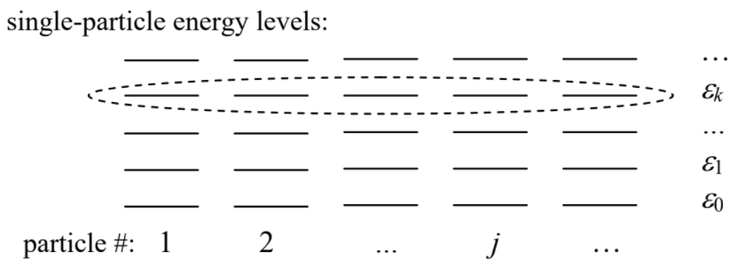
Now let us apply the general statistical distributions discussed above to a simple but very important case when the system we are considering consists of many similar particles whose explicit (“direct”) interaction is negligible. As a result, each particular energy value \(E_{m,N}\) of such a system may be represented as a sum of energies \(\varepsilon_k\) of the particles, where the index \(k\) numbers single-particle states – rather than those of the whole system, as the index \(m\) does.

Let us start with the classical limit. In classical mechanics, the energy quantization effects are negligible, i.e. there is a formally infinite number of quantum states \(k\) within each finite energy interval. However, it is convenient to keep, for the time being, the discrete-state language, with the understanding that the average number \(\langle N_k \rangle\) of particles in each of these states, usually called the state occupancy, is very small. In this case, we may apply the Gibbs distribution to the canonical ensemble of single particles, and hence use it with the substitution \(E_m \rightarrow \varepsilon_k\), so that Equation (\(2.4.7\)) becomes

Boltzmann distribution:

\[\boxed{ \langle N_k \rangle = c \text{ exp} \left\{ - \frac{\varepsilon_k}{T}\right\} <<1, } \label{111}\]

where the constant \(c\) should be found from the normalization condition:

\[\sum_k \langle N_k \rangle = 1.\]

This is the famous Boltzmann distribution.⁶³ Despite its formal similarity to the Gibbs distribution (\(2.4.7\)), let me emphasize the conceptual difference between these two important formulas. The Gibbs distribution describes the probability to find the whole system on one of its states with energy \(E_m\), and it is always valid – more exactly, for a canonical ensemble of systems in thermodynamic equilibrium. On the other hand, the Boltzmann distribution describes the occupancy of an energy level of a single particle, and, as we will see in just a minute, is valid for quantum particles only in the classical limit \(\langle N_k \rangle << 1\), even if they do not interact directly.

The last fact may be surprising, because it may seem that as soon as particles of the system are independent, nothing prevents us from using the Gibbs distribution to derive Equation (\ref{111}), regardless of the value of \(\langle N_k \rangle \). This is indeed true if the particles are distinguishable, i.e. may be distinguished from each other – say by their fixed spatial positions, or by the states of certain internal degrees of freedom (say, spin), or by any other “pencil mark”. However, it is an experimental fact that elementary particles of each particular type (say, electrons) are identical to each other, i.e. cannot be “pencil-marked”.⁶⁴ For such particles we have to be more careful: even if they do not interact explicitly, there is still some implicit dependence in their behavior, which is especially evident for the so-called fermions (elementary particles with semi-integer spin): they obey the Pauli exclusion principle that forbids two identical particles to be in the same quantum state, even if they do not interact explicitly.⁶⁵

Note that the term “the same quantum state” carries a heavy meaning load here. For example, if two particles are confined to stay at different spatial positions (say, reliably locked in different boxes), they are distinguishable even if they are internally identical. Thus the Pauli principle, as well as other particle identity effects such as the Bose-Einstein condensation to be discussed in the next chapter, are important only when identical particles may move in the same spatial region. To emphasize this fact, it is common to use, instead of “identical”, a more precise (though grammatically rather unpleasant) adjective indistinguishable.

In order to take these effects into account, let us examine statistical properties of a system of many non-interacting but indistinguishable particles (at the first stage of calculation, either fermions or bosons) in equilibrium, applying the grand canonical distribution (\(2.7.8\)) to a very unusual grand canonical ensemble: a subset of particles in the same quantum state \(k\) (Figure \(\PageIndex{1}\)).

Figure \(\PageIndex{1}\): The grand canonical ensemble of particles in the same quantum state with energy \(\varepsilon_k\) – schematically.

In this ensemble, the role of the environment may be played just by the set of particles in all other states \(k’ \neq k\), because due to infinitesimal interactions, the particles may gradually change their states. In the resulting equilibrium, the chemical potential \(\mu \) and temperature \(T\) of the system should not depend on the state number \(k\), though the grand thermodynamic potential \(\Omega_k\) of the chosen particle subset may. Replacing \(N\) with \(N_k\) – the particular (not average!) number of particles in the selected \(k^{th}\) state, and the particular energy value \(E_{m,N}\) with \(\varepsilon_k N_k\), we reduce the final form of Equation (\(2.7.8\)) to

\[\Omega_{k}=-T \ln \left(\sum_{N_{k}} \exp \left\{\frac{\mu N_{k}-\varepsilon_{k} N_{k}}{T}\right\}\right) \equiv-T \ln \left[\sum_{N_{k}}\left(\exp \left\{\frac{\mu-\varepsilon_{k}}{T}\right\}\right)^{N_{k}}\right] , \label{113}\]

where the summation should be carried out over all possible values of \(N_k\). For the final calculation of this sum, the elementary particle type is essential.

On one hand, for fermions, obeying the Pauli principle, the numbers \(N_k\) in Equation (\ref{113}) may take only two values, either 0 (the state \(k\) is unoccupied) or 1 (the state is occupied), and the summation gives

\[\Omega_{k}=-T \ln \left[\sum_{N_{k}=0,1}\left(\exp \left\{\frac{\mu-\varepsilon_{k}}{T}\right\}\right)^{N_{k}}\right] \equiv-T \ln \left(1+\exp \left\{\frac{\mu-\varepsilon_{k}}{T}\right\}\right). \label{114}\]

Now the state occupancy may be calculated from the last of Eqs. (\(1.5.13\)) – in this case, with the (average) \(N\) replaced with \(\langle N_k\rangle \):

Fermi-Dirac distribution:

\[\boxed{\langle N_k \rangle = - \left(\frac{\partial \Omega_k}{\partial \mu} \right)_{T, V} = \frac{1}{e^{(\varepsilon_k - \mu)/T} +1}. } \label{115}\]

This is the famous Fermi-Dirac distribution, derived in 1926 independently by Enrico Fermi and Paul Dirac.

On the other hand, bosons do not obey the Pauli principle, and for them the numbers \(N_k\) can take any non-negative integer values. In this case, Equation (\ref{113}) turns into the following equality:

\[\Omega_{k}=-T \ln \left[\sum_{N_{k}=0}^{\infty}\left(\exp \left\{\frac{\mu-\varepsilon_{k}}{T}\right\}\right)^{N_{k}}\right] \equiv-T \ln \sum_{N_{k}=0}^{\infty} \lambda^{N_{k}}, \text { with } \lambda \equiv \exp \left\{\frac{\mu-\varepsilon_{k}}{T}\right\}. \label{116}\]

This sum is just the usual geometric series, which converges if \(\lambda < 1\), giving

\[\Omega_k = -T \ln \frac{1}{1-\lambda} \equiv T \ln \left(1-\text{exp}\left\{\frac{\mu - \varepsilon_k}{T}\right\}\right), \quad \text{ for } \mu < \varepsilon_k. \label{117}\]

In this case, the average occupancy, again calculated using Equation (\(1.5.13\)) with \(N\) replaced with \(\langle N_k \rangle \), obeys the Bose-Einstein distribution,

Bose-Einstein distribution:

\[\boxed{ \langle N_k \rangle = - \left(\frac{\partial \Omega_k}{\partial \mu }\right)_{T,V} = \frac{1}{e^{\varepsilon_k - \mu)/T}-1}, \quad \text{ for } \mu < \varepsilon_k,} \label{118}\]

which was derived in 1924 by Satyendra Nath Bose (for the particular case \(\mu = 0\)) and generalized in 1925 by Albert Einstein for an arbitrary chemical potential. In particular, comparing Equation (\ref{118}) with Equation (\(2.5.15\)), we see that harmonic oscillator’s excitations,⁶⁶ each with energy \(\hbar \omega \), may be considered as bosons, with the chemical potential equal to zero. As a reminder, we have already obtained this equality (\(\mu = 0\)) in a different way – see Equation (\(2.6.14\)). Its physical interpretation is that the oscillator excitations may be created inside the system, so that there is no energy cost \(\mu\) of moving them into the system under consideration from its environment.

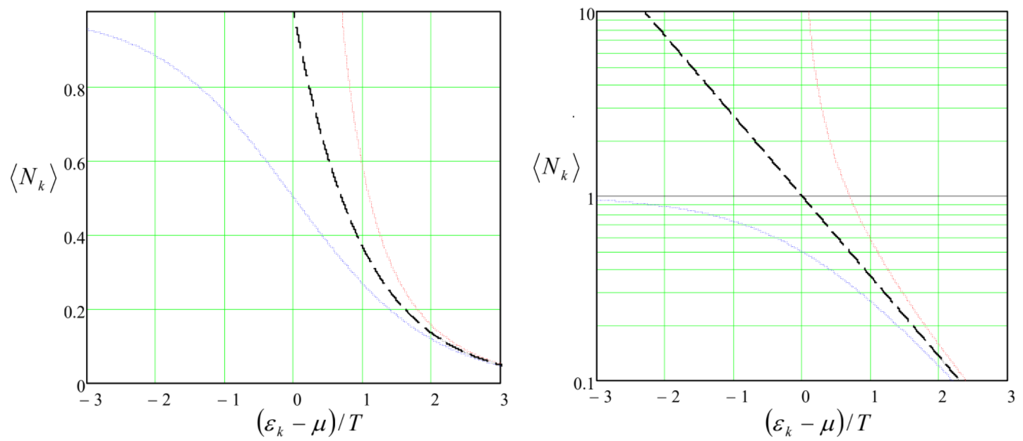
The simple form of Eqs. (\ref{115}) and (\ref{118}), and their similarity (besides “only” the difference of the signs before the unity in their denominators), is one of the most beautiful results of physics. This similarity, however, should not disguise the fact that the energy dependences of the occupancies \(\langle N_k\rangle\) given by these two formulas are very different – see their linear and semi-log plots in Figure \(\PageIndex{2}\).

In the Fermi-Dirac statistics, the level occupancy is not only finite, but below 1 at any energy, while in the Bose-Einstein it may be above 1, and diverges at \(\varepsilon_k \rightarrow \mu \).. However, as the temperature is increased, it eventually becomes much larger than the difference (\(\varepsilon_k – \mu \)). In this limit, \(\langle N_k\rangle << 1\), both quantum distributions coincide with each other, as well as with the classical Boltzmann distribution (\ref{111}) with \(c = \text{exp} \{\mu /T\}\):

Boltzmann distribution: identical particles

\[\boxed{\langle N_k \rangle \rightarrow \text{exp}\left\{\frac{\mu - \varepsilon_k}{T}\right\}, \quad \text{ for } \langle N_k \rangle \rightarrow 0. } \label{119}\]

This distribution (also shown in Figure \(\PageIndex{2}\)) may be, therefore, understood also as the high-temperature limit for indistinguishable particles of both sorts.

Figure \(\PageIndex{2}\): The Fermi-Dirac (blue line), Bose-Einstein (red line), and Boltzmann (dashed line) distributions for indistinguishable quantum particles. (The last distribution is valid only asymptotically, at \(\langle N_k \rangle << 1\).)

A natural question now is how to find the chemical potential \(\mu\) participating in Eqs. (\ref{115}), (\ref{118}), and (\ref{119}). In the grand canonical ensemble as such (Figure \(2.7.1\)), with the number of particles variable, the value of \(\mu\) is imposed by the system’s environment. However, both the Fermi-Dirac and Bose-Einstein distributions are also approximately applicable (in thermal equilibrium) to systems with a fixed but very large number \(N\) of particles. In these conditions, the role of the environment for some subset of \(N’ << N\) particles is essentially played by the remaining \(N – N’\) particles. In this case, \(\mu\) may be found by the calculation of \(\langle N\rangle\) from the corresponding probability distribution, and then requiring it to be equal to the genuine number of particles in the system. In the next section, we will perform such calculations for several particular systems.

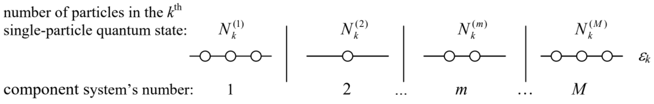
For that and other applications, it will be convenient for us to have ready formulas for the entropy \(S\) of a general (i.e. not necessarily equilibrium) state of systems of independent Fermi or Bose particles, expressed not as a function of \(W_m\) of the whole system, as in Equation (\(2.2.11\)), but via the occupancy numbers \(\langle N_k \rangle \). For that, let us consider an ensemble of composite systems, each consisting of \(M >> 1\) similar but distinct component systems, numbered by index \(m = 1, 2, ... M\), with independent (i.e. not directly interacting) particles. We will assume that though in each of \(M\) component systems the number \(N_k^{(m)}\) of particles in their \(k^{th}\) quantum state may be different (Figure \(\PageIndex{3}\)), their total number \(N_k^{(\Sigma )}\) in the composite system is fixed. As a result, the total energy of the composite system is fixed as well,

\[ \sum^M_{m=1} N_k^{(m)} = N_k^{(\Sigma)} = const, \quad E_k = \sum^M_{m=1} N_k^{(m)} \varepsilon_k = N_k^{(\Sigma)} \varepsilon_k = const, \label{120}\]

so that an ensemble of many such composite systems (with the same \(k\)), in equilibrium, is microcanonical.

Figure \(\PageIndex{3}\): A composite system of \(N_k^{(\Sigma )}\) particles in the \(k^{th}\) quantum state, distributed between \(M\) component systems.

According to Equation (\(2.2.5\)), the average entropy \(S_k\) per component system in this microcanonical ensemble may be calculated as

\[S_k = \lim_{M\to \infty} \frac{\ln M_k}{M}, \label{121}\]

where \(M_k\) is the number of possible different ways such a composite system (with fixed \(N_k^{(\Sigma )}\)) may be implemented. Let us start the calculation of \(M_k\) for Fermi particles – for which the Pauli principle is valid. Here the level occupancies \(N_k^{(m)}\) may be only equal to either 0 or 1, so that the distribution problem is solvable only if \(N_k^{(\Sigma )} \leq M\), and evidently equivalent to the choice of \(N_k^{(\Sigma )}\) balls (in arbitrary order) from the total number of \(M\) distinct balls. Comparing this formulation with the definition of the binomial coefficient,⁶⁷ we immediately get

\[M_k =^M C_{N_k^{(\Sigma)}} = \frac{M!}{(M-N_k^{(\Sigma)})!N_k^{(\Sigma)}!}. \label{122}\]

From here, using the Stirling formula (again, in its simplest form (\(2.2.9\))), we get

Fermions: entropy

\[\boxed{S_k = - \langle N_k \rangle \ln \langle N_k \rangle - (1- \langle N_k \rangle) \ln (1- \langle N_k \rangle), } \label{123}\]

where

\[\langle N_k \rangle \equiv \lim_{M\to \infty} \frac{N_k^{(\Sigma)}}{M}\label{124}\]

is exactly the average occupancy of the \(k^{th}\) single-particle state in each system, which was discussed earlier in this section. Since for a Fermi system, \(\langle N_k \rangle\) is always somewhere between 0 and 1, its entropy (\ref{123}) is always positive.

\[M_{k}=^{M+N_{k}-1} C_{M-1}=\frac{\left(M-1+N_{k}^{(\Sigma)}\right) !}{(M-1) ! N_{k}^{(\Sigma)} !}. \label{125}\]

Applying the Stirling formula (\(2.2.9\)) again, we get the following result,

Bosons: entropy

\[\boxed{S_k = -\langle N_k \rangle \ln \langle N_k \rangle + (1+\langle N_k \rangle) \ln (1+ \langle N_k \rangle), } \label{126}\]

which again differs from the Fermi case (\ref{123}) “only” by the signs in the second term, and is valid for any positive \(\langle N_k\rangle \).

Expressions (\ref{123}) and (\ref{126}) are valid for an arbitrary (possibly non-equilibrium) case; they may be also used for an alternative derivation of the Fermi-Dirac (\ref{115}) and Bose-Einstein (\ref{118}) distributions, which are valid only in equilibrium. For that, we may use the method of Lagrange multipliers, requiring (just like it was done in Sec. 2) the total entropy of a system of \(N\) independent, similar particles,

\[S = \sum_k S_k, \label{127}\]

considered as a function of state occupancies \(\langle N_k\rangle \), to attain its maximum, under the conditions of the fixed total number of particles \(N\) and total energy \(E\):

\[\sum_k \langle N_k \rangle = N = const, \quad \sum_k \langle N_k \rangle \varepsilon_k = E = const. \label{128}\]

The completion of this calculation is left for the reader’s exercise.

In the classical limit, when the average occupancies \(\langle N_k \rangle\) of all states are small, the Fermi and Bose expressions for \(S_k\) tend to the same limit

Boltzmann entropy:

\[\boxed{S_k = - \langle N_k \rangle \ln \langle N_k \rangle, \quad \text{ for } \langle N_k \rangle << 1.} \label{129}\]

This expression, frequently referred to as the Boltzmann (or “classical”) entropy, might be also obtained, for arbitrary \(\langle N_k \rangle \), directly from the functionally similar Equation (\(2.2.11\)), by considering an ensemble of systems, each consisting of just one classical particle, so that \(E_m \rightarrow \varepsilon_k\) and \(W_m \rightarrow \langle N_k \rangle \). Let me emphasize again that for indistinguishable particles, such identification is generally (i.e. at \(\langle N_k \rangle \sim 1\)) illegitimate even if the particles do not interact explicitly. As we will see in the next chapter, indistinguishability may affect the statistical properties of identical particles even in the classical limit.