
4.2: Continuous phase transitions
- Page ID
- 34714

As Figure \(4.1.2\) illustrates, if we fix pressure \(P\) in a system with a first-order phase transition, and start changing its temperature, then the complete crossing of the transition-point line, defined by the equation \(P_0(T) = P\), requires the insertion (or extraction) some non-zero latent heat \(\Lambda \). Eqs. (\(4.1.14\)) and (\(4.1.17\)) show that \(\Lambda\) is directly related to non-zero differences between the entropies and volumes of the two phases (at the same pressure). As we know from Chapter 1, both \(S\) and \(V\) may be represented as the first derivatives of appropriate thermodynamic potentials. This is why P. Ehrenfest called such transitions, involving jumps of potentials' first derivatives, the first-order phase transitions.
On the other hand, there are phase transitions that have no first derivative jumps at the transition temperature \(T_c\), so that the temperature point may be clearly marked, for example, by a jump of the second derivative of a thermodynamic potential – for example, the derivative \(\partial C/\partial T\) which, according to Equation (\(1.4.1\)), equals to \(\partial^2E/\partial T^2\). In the initial Ehrenfest classification, this was an example of a second-order phase transition. However, most features of such phase transitions are also pertinent to some systems in which the second derivatives of potentials are continuous as well. Due to this reason, I will use a more recent terminology (suggested in 1967 by M. Fisher), in which all phase transitions with \(\Lambda = 0\) are called continuous.
Most (though not all) continuous phase transitions result from particle interactions. Here are some representative examples:
(i) At temperatures above \(\sim\) 490 K, the crystal lattice of barium titanate \((\ce{BaTiO3})\) is cubic, with a Ba ion in the center of each Ti-cornered cube (or vice versa) – see Figure \(\PageIndex{1a}\). However, as the temperature is being lowered below that critical value, the sublattice of Ba ions starts moving along one of six sides of the \(\ce{TiO3}\) sublattice, leading to a small deformation of both lattices – which become tetragonal. This is a typical example of a structural transition, in this particular case combined with a ferroelectric transition, because (due to the positive electric charge of the Ba ions) below the critical temperature the \(\ce{BaTiO3}\) crystal acquires a spontaneous electric polarization even in the absence of external electric field.
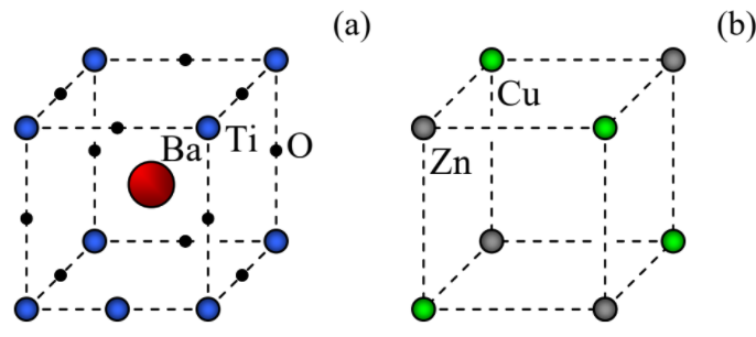
(ii) A different kind of phase transition happens, for example, in Cu\(_x\)Zn\(_{1-x}\) alloys – so-called brasses. Their crystal lattice is always cubic, but above certain critical temperature \(T_c\) (which depends on \(x\)) any of its nodes may be occupied by either a copper or a zinc atom, at random. At \(T < T_c\), a trend toward ordered atom alternation arises, and at low temperatures, the atoms are fully ordered, as shown in Figure \(\PageIndex{1b}\) for the stoichiometric case \(x = 0.5\). This is a good example of an order-disorder transition.
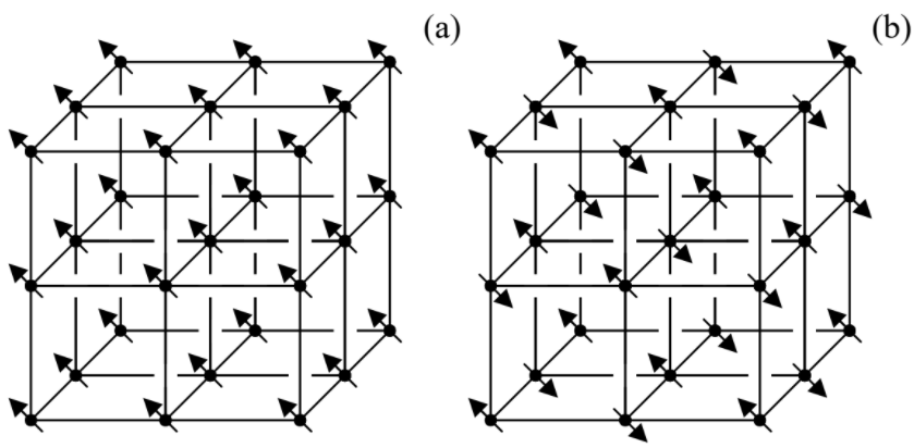
(iii) At ferromagnetic transitions (such as the one taking place, for example, in Fe at 1,388 K) and antiferromagnetic transitions (e.g., in MnO at 116 K), lowering of temperature below the critical value16 does not change atom positions substantially, but results in a partial ordering of atomic spins, eventually leading to their full ordering (Figure \(\PageIndex{2}\)).
Note that, as it follows from Eqs. (\(1.1.1\))-(\(1.1.5\)), at ferroelectric transitions the role of pressure is played by the external electric field \(\pmb{\mathscr{E}}\), and at the ferromagnetic transitions, by the external magnetic field \(\pmb{\mathscr{H}}\). As we will see very soon, even in systems with continuous phase transitions, a gradual change of such an external field, at a fixed temperature, may induce jumps between metastable states, similar to those in systems with first-order phase transitions (see, e.g., the dashed arrows in Figure \(4.1.2\)), with non-zero decreases of the appropriate free energy.
Besides these standard examples, some other threshold phenomena, such as the formation of a coherent optical field in a laser, and even the self-excitation of oscillators with negative damping (see, e.g., CM Sec. 5.4), may be treated, at certain conditions, as continuous phase transitions.17
The general feature of all these transitions is the gradual formation, at \(T < T_c\), of certain ordering, which may be characterized by some order parameter \(\eta \neq 0\). The simplest example of such an order parameter is the magnetization at the ferromagnetic transitions, and this is why the continuous phase transitions are usually discussed on certain models of ferromagnetism. (I will follow this tradition, while mentioning in passing other important cases that require a substantial modification of the theory.) Most of such models are defined on an infinite 3D cubic lattice (see, e.g., Figure \(\PageIndex{2}\)), with evident generalizations to lower dimensions. For example, the Heisenberg model of a ferromagnet (suggested in 1928) is defined by the following Hamiltonian:
Heisenberg model:
\[\boxed{ \hat{H} = -J \sum_{\{k,k'\}} \hat{\boldsymbol{\sigma}}_k \cdot \hat{\boldsymbol{\sigma}}_{k'}-\sum_k\mathbf{h}\cdot \hat{\boldsymbol{\sigma}}_k,}\label{21}\]
where \(\hat{\boldsymbol{\sigma}}_k\) is the Pauli vector operator18 acting on the \(k^{th}\) spin, and \(\mathbf{h}\) is the normalized external magnetic field:
\[ \mathbf{h} \equiv \mathscr{m}_0\mu_0\pmb{\mathscr{H}} . \label{22}\]
Ising model:
\[\boxed{E_m = -J \sum_{\{k,k'\}}s_ks_{k'}-h\sum_ks_k.} \label{23}\]
Evidently, if \(T = 0\) and \(h = 0\), the lowest possible energy,
\[E_{min} = −JNd , \label{24}\]
where \(d\) is the lattice dimensionality, is achieved in the “ferromagnetic” phase in which all spins \(s_k\) are equal to either +1 or –1, so that \(\langle s_k \rangle = \pm 1\) as well. On the other hand, at \(J = 0\), the spins are independent, and if \(h = 0\) as well, all \(s_k\) are completely random, with the 50% probability to take either of values \(\pm 1\), so that \(\langle s_k \rangle = 0\). Hence in the general case (with arbitrary \(J\) and \(h\)), we may use the average
Ising model: order parameter
\[\boxed{\eta \equiv \langle s_k \rangle} \label{25}\]
as a good measure of spin ordering, i.e. as the order parameter. Since in a real ferromagnet, each spin carries a magnetic moment, the order parameter \(\eta\) is proportional to the Cartesian component of the system's magnetization, in the direction of the applied magnetic field.
Now that the Ising model gave us a very clear illustration of the order parameter, let me use this notion for quantitative characterization of continuous phase transitions. Due to the difficulty of theoretical analyses of most models of the transitions at arbitrary temperatures, their theoretical discussions are focused mostly on a close vicinity of the critical point \(T_c\). Both experiment and theory show that in the absence of an external field, the function \(\eta (T)\) is close to a certain power,
\[\eta \propto \tau^{\beta}, \quad \text{ for } \tau > 0, \text{ i.e. } T < T_c \label{26}\]
of the small deviation from the critical temperature – which is conveniently normalized as
\[\tau \equiv \frac{T_c-T}{T_c}.\label{27}\]
\[c_h \propto |\tau |^{-\alpha}. \label{28}\]
\[\chi \equiv \frac{\partial \eta}{\partial h} \mid_{h=0} \propto |\tau |^{-\gamma}. \label{29}\]
Two other important critical exponents, \(\zeta\) and \(\nu\), describe the temperature behavior of the correlation function \(\langle s_ks_{k'}\rangle \), whose dependence on the distance \(r_{kk'}\) between two spins may be well fitted by the following law,
\[\left\langle s_{k} s_{k^{\prime}}\right\rangle \propto \frac{1}{r_{k k^{\prime}}{ }^{d-2+\zeta}} \exp \left\{-\frac{r_{k k^{\prime}}}{r_{\mathrm{c}}}\right\}, \label{30}\]
with the correlation radius
\[r_c \propto |\tau |^{-\nu }.\label{31}\]
Finally, three more critical exponents, usually denoted \(\varepsilon \), \(\delta \), and \(\mu \), describe the external field dependences of, respectively, \(c\), \(\eta \), and \(r_c\) at \(\tau > 0\). For example, \(\delta\) is defined as
\[\eta \propto h^{1/\delta}. \label{32}\]
(Other field exponents are used less frequently, and for their discussion, the interested reader is referred to the special literature that was cited above.)
The leftmost column of Table \(\PageIndex{1}\) shows the ranges of experimental values of the critical exponents for various 3D physical systems featuring continuous phase transitions. One can see that their values vary from system to system, leaving no hope for a universal theory that would describe them all exactly. However, certain combinations of the exponents are much more reproducible – see the four bottom lines of the table.
Table \(\PageIndex{1}\): Major critical exponents of continuous phase transitions
|
Exponents and combinations |
Experimental range (3D)\(^{(a)}\) |
Landau's theory |
2D Ising model |
3D Ising model |
3D Heisenberg Model\(^{(d)}\) |
|
\(\alpha\) |
0 – 0.14 |
\(0^{(b)}\) |
\(^{(c)}\) |
0.12 |
–0.14 |
|
\(\beta\) |
0.32 – 0.39 |
1/2 |
1/8 |
0.31 |
0.3 |
|
\(\gamma\) |
1.3 – 1.4 |
1 |
7/4 |
1.25 |
1.4 |
|
\(\delta\) |
4-5 |
3 |
15 |
5 |
? |
|
\(\nu \) |
0.6 – 0.7 |
1/2 |
1 |
0.64 |
0.7 |
|
\(\zeta\) |
0.05 |
0 |
1/4 |
0.05 |
0.04 |
|
\((\alpha + 2\beta + \gamma )/2 \) |
\(1.00 \pm 0.005\) |
1 |
1 |
1 |
1 |
|
\(\delta – \gamma /\beta\) |
\(0.93 \pm 0.08\) |
1 |
1 |
1 |
? |
|
\((2 – \zeta )\nu /\gamma\) |
\(1.02 \pm 0.05\) |
1 |
1 |
1 |
1 |
|
\((2 – \alpha )/\nu d\) |
? |
\(4/d\) |
1 |
1 |
1 |
(a) Experimental data are from the monograph by A. Patashinskii and V. Pokrovskii, cited above.
(b) Discontinuity at \(\tau = 0\) – see below.
(c) Instead of following Equation (\ref{28}), in this case \(c_h\) diverges as \(\ln|\tau |\).
(d) With the order parameter \(\eta\) defined as \(\langle \boldsymbol{\sigma}_j \cdot \pmb{\mathscr{B}}\rangle /\mathscr{B}\).
Historically the first (and perhaps the most fundamental) of these universal relations was derived in 1963 by J. Essam and M. Fisher:
\[ \alpha + 2\beta + \gamma = 2 . \label{33}\]
It may be proved, for example, by finding the temperature dependence of the magnetic field value, \(h_{\tau }\), that changes the order parameter by the same amount as a finite temperature deviation \(\tau > 0\) gives at \(h = 0\). Comparing Eqs. (\ref{26}) and (\ref{29}), we get
\[h_{\tau} \propto \tau^{\beta + \gamma}. \label{34}\]
In order to estimate the thermal effect on \(F\), let me first elaborate a bit more on the useful thermodynamic formula already mentioned in Sec. 1.3:
\[C_X = T \left(\frac{\partial S}{\partial T} \right)_X, \label{35}\]
where \(X\) means the variable(s) maintained constant at the temperature variation. In the standard “\(P-V\)” thermodynamics, we may use Eqs. (\(1.4.12\)) for \(X = V\), and Eqs. (\(1.4.16\)) for \(X = P\), to write
\[C_{V}=T\left(\frac{\partial S}{\partial T}\right)_{V, N}=-T\left(\frac{\partial^{2} F}{\partial T^{2}}\right)_{V, N}, \quad C_{P}=T\left(\frac{\partial S}{\partial T}\right)_{P, N}=-T\left(\frac{\partial^{2} G}{\partial T^{2}}\right)_{P, N} . \label{36}\]
As was just discussed, in the ferromagnetic models of the type (\ref{21}) or (\ref{23}), at a constant field \(h\), the role of \(G\) is played by \(F\), so that Equation (\ref{35}) yields
\[C_{h}=T\left(\frac{\partial S}{\partial T}\right)_{h, N}=-T\left(\frac{\partial^{2} F}{\partial T^{2}}\right)_{h, N}. \label{37}\]
The last form of this relation means that \(F\) may be found by double integration of \((–C_h/T)\) over temperature. With Equation (\ref{28}) for \(c_h \propto C_h\), this means that near \(T_c\), the free energy scales as the double integral of \(c_h \propto \tau^{–\alpha}\) over \(\tau \). In the limit \(\tau << 1\), the factor \(T\) may be treated as a constant; as a result, the change of \(F\) due to \(\tau > 0\) alone scales as \(\tau^{(2 – \alpha )}\). Requiring this change to be proportional to the same power of \(\tau\) as the field-induced part of the energy, we finally get the Essam-Fisher relation (\ref{33}).
Using similar reasoning, it is straightforward to derive a few other universal relations of critical exponents, including the Widom relation,
\[\delta - \frac{\gamma}{\beta} =1, \label{38}\]
\[ \nu (2 − \zeta ) = \gamma . \label{39}\]
\[ \nu d = 2 −\alpha . \label{40}\]
The second column of Table \(\PageIndex{1}\) shows that at least three of these relations are in a very reasonable agreement with experiment, so that we may use their set as a testbed for various theoretical approaches to continuous phase transitions.