4.3: Landau’s mean-field theory

The highest-level approach to continuous phase transitions, formally not based on any particular microscopic model (though in fact implying either the Ising model (\(4.2.3\)) or one of its siblings), is the mean-field theory developed in 1937 by L. Landau, on the basis of prior ideas by P. Weiss – to be discussed in the next section. The main idea of this phenomenological approach is to represent the free energy's change \(\Delta F\) at the phase transition as an explicit function of the order parameter \(\eta\) (\(4.2.5\)). Since at \(T \rightarrow T_c\), the order parameter has to tend to zero, this change,

\[\Delta F \equiv F(T)-F(T_c),\label{41}\]

may be expanded into the Taylor series in \(\eta \), and only a few, most important first terms of that expansion retained. In order to keep the symmetry between two possible signs of the order parameter (i.e. between two possible spin directions in the Ising model) in the absence of external field, at \(h = 0\) this expansion should include only even powers of \(\eta \):

\[ \left.\left.\Delta f\right|_{h=0} \equiv \frac{\Delta F}{V}\right|_{h=0}=A(T) \eta^{2}+\frac{1}{2} B(T) \eta^{4}+\ldots, \quad \text { at } T \approx T_{c} . \label{42}\]

As Figure \(\PageIndex{1}\) shows, at \(A(T) < 0\), and \(B(T) > 0\), these two terms are sufficient to describe the minimum of the free energy at \(\eta 2 > 0\), i.e. to calculate stationary values of the order parameter; this is why Landau's theory ignores higher terms of the Taylor expansion – which are much smaller at \(\eta \rightarrow 0\).

Figure \(\PageIndex{1}\): The Landau free energy (\ref{42}) as a function of (a) \(\eta\) and (b) \(\eta^2\), for two signs of the coefficient \(A(T)\), both for \(B(T) > 0\).

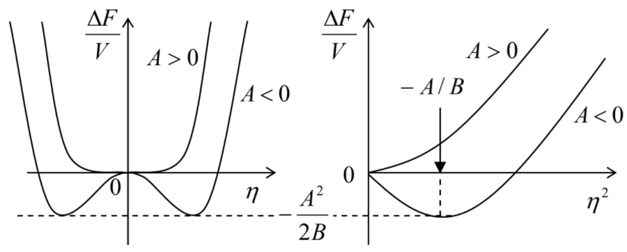
Now let us discuss the temperature dependencies of the coefficients \(A\) and \(B\). As Equation (\ref{42}) shows, first of all, the coefficient \(B(T)\) has to be positive for any sign of \(\tau \propto (T_c – T)\), to ensure the equilibrium at a finite value of \(\eta^2\). Thus, it is reasonable to ignore the temperature dependence of \(B\) near the critical temperature altogether, i.e. use the approximation

\[ B(T) = b > 0. \label{43}\]

On the other hand, as Figure \(\PageIndex{1}\) shows, the coefficient \(A(T)\) has to change sign at \(T = T_c\), to be positive at \(T > T_c\) and negative at \(T < T_c\), to ensure the transition from \(\eta = 0\) at \(T > T_c\) to a certain non-zero value of the order parameter at \(T < T_c\). Assuming that \(A\) is a smooth function of temperature, we may approximate it by the leading term of its Taylor expansion in \(\tau \):

\[ A(T) = −a\tau , \quad \text{ with } a > 0, \label{44}\]

so that Equation (\ref{42}) becomes

\[ \left. \Delta f \right|_{h=0} −a\tau \eta^2 + \frac{1}{2}b\eta^4 . \label{45}\]

In this rudimentary form, the Landau theory may look almost trivial, and its main strength is the possibility of its straightforward extension to the effects of the external field and of spatial variations of the order parameter. First, as the field terms in Eqs. (\(4.2.1\)) or (\(4.2.3\)) show, the applied field gives such systems, on average, the energy addition of \(–h\eta\) per particle, i.e. \(–nh\eta\) per unit volume, where \(n\) is the particle density. Second, since according to Equation (\(4.2.11\)) (with \(\nu > 0\), see Table \(4.2.1\)) the correlation radius diverges at \(\tau \rightarrow 0\), in this limit the spatial variations of the order parameter should be slow, \(|\nabla \eta |\rightarrow 0\). Hence, the effects of the gradient on \(\Delta F\) may be approximated by the first non-zero term of its expansion into the Taylor series in \((\nabla \eta )^2\).²⁶ As a result, Equation (\ref{45}) may be generalized as

Landau theory: free energy

\[\boxed{\Delta F = \int \Delta fd^3 r, \quad \text{ with } \Delta f = −a\tau \eta^2 + \frac{1}{2} b\eta^4 − nh\eta + c ( \nabla \eta )^2, } \label{46}\]

where \(c\) is a coefficient independent of \(\eta \). To avoid the unphysical effect of spontaneous formation of spatial variations of the order parameter, that factor has to be positive at all temperatures and hence may be taken for a constant in a small vicinity of \(T_c\) – the only region where Equation (\ref{46}) may be expected to provide quantitatively correct results.

Let us find out what critical exponents are predicted by this phenomenological approach. First of all, we may find the equilibrium values of the order parameter from the condition of \(F\) having a minimum, \(\partial F/\partial \eta = 0\). At \(h = 0\), it is easier to use the equivalent equation \(\partial F/\partial (\eta 2) = 0\), where \(F\) is given by Equation (\ref{45}) – see Figure \(\PageIndex{1b}\). This immediately yields

\[|\eta|= \begin{cases}(a \tau / b)^{1 / 2}, & \text { for } \tau>0 \\ 0, & \text { for } \tau<0.\end{cases} \label{47}\]

Comparing this result with Equation (\(4.2.6\)), we see that in the Landau theory, \(\beta = 1/2\). Next, plugging the result (\ref{47}) back into Equation (\ref{45}), for the equilibrium (minimal) value of the free energy, we get

\[\Delta f = \begin{cases} -a^2 \tau^2 / 2b, & \text { for } \tau>0 \\ 0, & \text { for } \tau<0.\end{cases} \label{48}\]

From here and Equation (\(4.2.17\)), the specific heat,

\[\frac{C_h}{V} = \begin{cases} a^2 / b T_c, & \text { for } \tau>0 \\ 0, & \text { for } \tau<0,\end{cases} \label{49}\]

has, at the critical point, a discontinuity rather than a singularity, so that we need to prescribe zero value to the critical exponent \(\alpha \).

In the presence of a uniform field, the equilibrium order parameter should be found from the condition \(\partial f/\partial \eta = 0\) applied to Equation (\ref{46}) with \(\nabla \eta = 0\), giving

\[\frac{\partial f}{\partial \eta} \equiv -2 a \tau \eta +2 b \eta^3 - nh = 0. \label{50}\]

In the limit of a small order parameter, \(\eta \rightarrow 0\), the term with \(\eta 3\) is negligible, and Equation (\ref{50}) gives

\[\eta = - \frac{nh}{2a \tau},\label{51}\]

so that according to Equation (\(4.2.9\)), \(\gamma = 1\). On the other hand, at \(\tau = 0\) (or at relatively high fields at other temperatures), the cubic term in Equation (\ref{50}) is much larger than the linear one, and this equation yields

\[\eta = \left( \frac{nh}{2b}\right)^{1/3}, \label{52}\]

so that comparison with Equation (\(4.2.12\)) yields \(\delta = 3\). Finally, according to Equation (\(4.2.10\)), the last term in Equation (\ref{46}) scales as \(c\eta^2/r_c^2\). (If \(r_c \neq \infty \), the effects of the pre-exponential factor in Equation (\(4.2.10\)) are negligible.) As a result, the gradient term's contribution is comparable²⁷ with the two leading terms in \(\Delta f\) (which, according to Equation (\ref{47}), are of the same order), if

\[r_c \approx \left(\frac{c}{a|\tau |} \right)^{1/2}, \label{53}\]

so that according to the definition (\(4.2.11\)) of the critical exponent \(\nu \), in the Landau theory it is equal to 1/2.

The third column in Table \(4.2.1\) summarizes the critical exponents and their combinations in Landau's theory. It shows that these values are somewhat out of the experimental ranges, and while some of their “universal” relations are correct, some are not; for example, the Josephson relation would be only correct at \(d = 4\) (not the most realistic spatial dimensionality :-) The main reason for this disappointing result is that describing the spin interaction with the field, the Landau mean-field theory neglects spin randomness, i.e. fluctuations. Though a quantitative theory of fluctuations will be discussed only in the next chapter, we can readily perform their crude estimate. Looking at Equation (\ref{46}), we see that its first term is a quadratic function of the effective “half-degree of freedom”, \(\eta \). Hence per the equipartition theorem (\(2.2.10\)), we may expect that the average square of its thermal fluctuations, within a \(d\)-dimensional volume with a linear size of the order of \(r_c\), should be of the order of \(T/2\) (close to the critical temperature, \(T_c/2\) is a good enough approximation):

\[a| \tau | \langle \tilde{\eta} \rangle r^d_c \sim \frac{T_c}{2}. \label{54}\]

In order to be negligible, the variance has to be small in comparison with the average \(\eta 2 \sim a\tau /b\) – see Equation (\ref{47}). Plugging in the \(\tau \)-dependences of the operands of this relation, and values of the critical exponents in the Landau theory, for \(\tau > 0\) we get the so-called Levanyuk-Ginzburg criterion of its validity:

\[\frac{T_c}{2a \tau} \left(\frac{a\tau }{c} \right)^{d/2} << \frac{a\tau}{b}. \label{55}\]

We see that for any realistic dimensionality, \(d < 4\), at \(\tau \rightarrow 0\) the order parameter's fluctuations grow faster than its average value, and hence the theory becomes invalid.

Thus the Landau mean-field theory is not a perfect approach to finding critical indices at continuous phase transitions in Ising-type systems with their next-neighbor interactions between the particles. Despite that fact, this theory is very much valued because of the following reason. Any long range interactions between particles increase the correlation radius \(r_c\), and hence suppress the order parameter fluctuations. As one example, at laser self-excitation, the emerging coherent optical field couples essentially all photon-emitting particles in the electromagnetic cavity (resonator). As another example, in superconductors the role of the correlation radius is played by the Cooper-pair size \(\xi_0\), which is typically of the order of \(10^{-6}\) m, i.e. much larger than the average distance between the pairs (\(\sim 10^{-8}\) m). As a result, the mean-field theory remains valid at all temperatures besides an extremely small temperature interval near \(T_c\) – for bulk superconductors, of the order of \(10^{-6}\) K.

Another strength of Landau's classical mean-field theory (\ref{46}) is that it may be readily generalized for a description of Bose-Einstein condensates, i.e. quantum fluids. Of those generalizations, the most famous is the Ginzburg-Landau theory of superconductivity. It was developed in 1950, i.e. even before the microscopic-level explanation of this phenomenon by J. Bardeen, L. Cooper, and R. Schrieffer in 1956-57. In this theory, the real order parameter \(\eta\) is replaced with the modulus of a complex function \(\psi \), physically the wavefunction of the coherent Bose-Einstein condensate of Cooper pairs. Since each pair carries the electric charge \(q = –2e\) and has zero spin, it interacts with the magnetic field in a way different from that described by the Heisenberg or Ising models. Namely, as was already discussed in Sec. 3.4, in the magnetic field, the del operator \(\nabla\) in Equation (\ref{46}) has to be complemented with the term \(–i(q/\hbar )\mathbf{A}\), where \(\mathbf{A}\) is the vector potential of the total magnetic field \(\pmb{\mathscr{B}} = \nabla \times \mathbf{A}\), including not only the external magnetic field \(\pmb{\mathscr{H}}\) but also the field induced by the supercurrent itself. With the account for the well-known formula for the magnetic field energy, Equation (\ref{46}) is now replaced with

GL theory: free energy

\[\boxed{\Delta f=-a \tau|\psi|^{2}+\frac{1}{2} b|\psi|^{4}-\frac{\hbar^{2}}{2 m}\left|\left(\nabla-i \frac{q}{\hbar} \mathbf{A}\right) \psi\right|^{2}+\frac{\mathscr{B}^{2}}{2 \mu_{0}},}\label{56}\]

where \(m\) is a phenomenological coefficient rather than the actual particle's mass.

The variational minimization of the resulting Gibbs energy density \(\Delta g \equiv \Delta f – \mu_0 \pmb{\mathscr{H}} \cdot \pmb{\mathscr{M}} \equiv \Delta f – \pmb{\mathscr{H}} \cdot \pmb{\mathscr{B}} + \) const²⁸ over the variables \(\psi\) and \(\pmb{\mathscr{B}}\) (which is suggested for reader's exercise) yields two differential equations:

GL equations:

\[\boxed{\frac{\nabla \times \mathscr{B}}{\mu_{0}}=q \frac{i \hbar}{2 m}\left[\psi\left(\nabla-i \frac{q}{\hbar} \mathbf{A}\right) \psi^{*}-\text { c.c. }\right], }\label{57a}\]

\[\boxed{a \tau \psi=b|\psi|^{2} \psi-\frac{\hbar^{2}}{2 m}\left(\nabla-i \frac{q}{\hbar} \mathbf{A}\right)^{2} \psi . } \label{57b}\]

The first of these Ginzburg-Landau equations (\ref{57a}) should be no big surprise for the reader, because according to the Maxwell equations, in magnetostatics the left-hand side of Equation (\ref{57a}) has to be equal to the electric current density, while its right-hand side is the usual quantum-mechanical probability current density multiplied by \(q\), i.e. the density \(\mathbf{j}\) of the electric current of the Cooper pair condensate. (Indeed, after plugging \(\psi = n^{1/2}\text{exp}\{i\phi \}\) into that expression, we come back to Equation (\(3.4.15\)) which, as we already know, explains such macroscopic quantum phenomena as the magnetic flux quantization and the Meissner-Ochsenfeld effect.)

However, Equation (\ref{57b}) is new for us – at least for this course.²⁹ Since the last term on its right-hand side is the standard wave-mechanical expression for the kinetic energy of a particle in the presence of a magnetic field,³⁰ if this term dominates that side of the equation, Equation (\ref{57b}) is reduced to the stationary Schrödinger equation \(E\psi = \hat{H}\psi \), for the ground state of free Cooper pairs, with the total energy \(E = a\tau \). However, in contrast to the usual (single-particle) Schrödinger equation, in which \(|\psi |\) is determined by the normalization condition, the Cooper pair condensate density \(n = |\psi |^2\) is determined by the thermodynamic balance of the condensate with the ensemble of “normal” (unpaired) electrons, which plays the role of the uncondensed part of the particles in the usual Bose-Einstein condensate – see Sec. 3.4. In Equation (\ref{57b}), such balance is enforced by the first term \(b|\psi |^2\psi\) on the right-hand side. As we have already seen, in the absence of magnetic field and spatial gradients, such term yields \(|\psi | \propto \tau^{1/2} \propto (T_c – T)^{1/2}\) – see Equation (\ref{47}).

As a parenthetic remark, from the mathematical standpoint, the term \(b|\psi |^2\psi \), which is nonlinear in \(\psi \), makes Equation (\ref{57b}) a member of the family of the so-called nonlinear Schrödinger equations. Another member of this family, important for physics, is the Gross-Pitaevskii equation,

Gross-Pitaevskii equation:

\[\boxed{a \tau \psi = b | \psi |^2 \psi - \frac{\hbar^2}{2m} \nabla^2 \psi + U(\mathbf{r})\psi , } \label{58}\]

which gives a reasonable (albeit approximate) description of gradient and field effects on Bose-Einstein condensates of electrically neutral atoms at \(T \approx T_c\). The differences between Eqs. (\ref{58}) and (\ref{57a}-\ref{57b}) reflect, first, the zero electric charge \(q\) of the atoms (so that Equation (\ref{57a}) becomes trivial) and, second, the fact that the atoms forming the condensates may be readily placed in external potentials \(U(\mathbf{r}) \neq\) const (including the time-averaged potentials of optical traps – see EM Chapter 7), while in superconductors such potential profiles are much harder to create due to the screening of external electric and optical fields by conductors – see, e.g., EM Sec. 2.1.

Returning to the discussion of Equation (\ref{57b}), it is easy to see that its last term increases as either the external magnetic field or the density of current passed through a superconductor are increased, increasing the vector potential. In the Ginzburg-Landau equation, this increase is matched by a corresponding decrease of \(|\psi |^2\), i.e. of the condensate density \(n\), until it is completely suppressed. This balance describes the well-documented effect of superconductivity suppression by an external magnetic field and/or the supercurrent passed through the sample. Moreover, together with Equation (\ref{57a}), naturally describing the flux quantization (see Sec. 3.4), Equation (\ref{57b}) explains the existence of the so-called Abrikosov vortices – thin magnetic-field tubes, each carrying one quantum \(\Phi_0\) of magnetic flux – see Equation (\(3.4.17\)). At the core part of the vortex, \(|\psi |^2\) is suppressed (down to zero at its central line) by the persistent, dissipation-free current of the superconducting condensate, which circulates around the core and screens the rest of the superconductor from the magnetic field carried by the vortex.³¹ The penetration of such vortices into the so-called type-II superconductors enables them to sustain zero dc resistance up to very high magnetic fields of the order of 20 T, and as a result, to be used in very compact magnets – including those used for beam bending in particle accelerators.

Moreover, generalizing Eqs. (\ref{57a}-\ref{57b}) to the time-dependent case, just as it is done with the usual Schrödinger equation, one can describe other fascinating quantum macroscopic phenomena such as the Josephson effects, including the generation of oscillations with frequency \(\omega_J = (q/\hbar )\mathscr{V}\) by weak links between two superconductors, biased by dc voltage \(\mathscr{V}\). Unfortunately, time/space restrictions do not allow me to discuss these effects in any detail in this course, and I have to refer the reader to special literature.³² Let me only note that in the limit \(T \rightarrow T_c\), and for not extremely pure superconductor crystals (in which the so-called non-local transport phenomena may be important), the Ginzburg-Landau equations are exact, and may be derived (and their parameters \(T_c\), \(a\), \(b\), \(q\), and \(m\) determined) from the standard “microscopic” theory of superconductivity, based on the initial work by Bardeen, Cooper, and Schrieffer.³³ Most importantly, such derivation proves that \(q = –2e\) – the electric charge of a single Cooper pair.