6.5: Thermoelectric effects

Now let us return to our analysis of kinetic effects using the Boltzmann-RTA equation, and extend it even further, to the effects of a non-zero (albeit small) temperature gradient. Again, since for any of the statistics (\(6.2.2\)), the average occupancy \(\langle N(\varepsilon )\rangle\) is a function of just one combination of all its arguments, \(\xi \equiv (\varepsilon – \mu )/T\), its partial derivatives obey not only Equation (\(6.3.2\)), but also the following relation:

\[\frac{\partial \langle N (\varepsilon ) \rangle}{\partial T} = - \frac{\varepsilon - \mu}{T^2} \frac{\partial \langle N (\varepsilon ) \rangle}{\partial \xi } = \frac{\varepsilon - \mu }{T} \frac{\partial \langle N (\varepsilon ) \rangle}{\partial \mu }. \label{94}\]

As a result, Equation (\(6.3.3\)) is generalized as

\[\nabla w_0 = -\frac{\partial w_0}{\partial \varepsilon} \left( \nabla \mu + \frac{\varepsilon - \mu}{T} \nabla T \right),\label{95}\]

giving the following generalization of Equation (\(6.3.4\)):

\[\tilde{w} = \tau \frac{\partial w_0}{\partial \varepsilon} \mathbf{v} \cdot \left( \nabla \mu ' + \frac{\varepsilon - \mu}{T} \nabla T \right).\label{96}\]

Now, calculating current density as in Sec. 3, we get the result that is traditionally represented as

\[ \mathbf{j} = \sigma \left( - \frac{\nabla \mu ' }{q} \right) + \sigma \mathcal{S} (-\nabla T), \label{97}\]

where the constant \(\mathcal{S}\), called the Seebeck coefficient⁶¹ (or the “thermoelectric power”, or just “thermopower”) is given by the following relation:

Seebeck coefficient:

\[\boxed{ \sigma \mathcal{S} = \frac{gq\tau}{(2\pi\hbar)^3}\frac{4\pi}{3} \int^{\infty}_0 (8m\varepsilon^3)^{1/2} \frac{(\varepsilon - \mu )}{T} \left[ - \frac{\partial \langle N (\varepsilon ) \rangle }{\partial \varepsilon} \right] d\varepsilon . } \label{98}\]

Working out this integral for the most important case of a degenerate Fermi gas, with \(T << \varepsilon_F\), we have to be careful because the center of the sharp peak of the last factor under the integral coincides with the zero point of the previous factor, \((\varepsilon – \mu )/T\). This uncertainty may be resolved using the Sommerfeld expansion formula (\(3.3.8\)). Indeed, for a smooth function \(f(\varepsilon )\) obeying Equation (\(3.3.9\)), so that \(f(0) = 0\), we may use Equation (\(3.3.10\)) to rewrite Equation (\(3.3.8\)) as

\[\int^{\infty}_0 f(\varepsilon ) \left[ - \frac{\partial \langle N (\varepsilon ) \rangle }{\partial \varepsilon} \right] d\varepsilon = f(\mu ) + \frac{\pi^2T^2}{6} \left. \frac{d^2f(\varepsilon )}{d\varepsilon^2} \right|_{\varepsilon = \mu } . \label{99}\]

In particular, for working out the integral (\ref{98}), we may take \(f(\varepsilon ) \equiv (8m\varepsilon^3)^{1/2}(\varepsilon – \mu )/T\). (For this function, the condition \(f(0) = 0\) is evidently satisfied.) Then \(f(\mu ) = 0\), \(d^2f/d\varepsilon^2|_{\varepsilon =\mu} = 3(8m\mu )^{1/2}/T \approx 3(8m\varepsilon_F)^{1/2}/T\), and Equation (\ref{98}) yields

\[\sigma \mathcal{S} = \frac{gq\tau}{(2\pi \hbar )^3} \frac{4\pi}{3}\frac{\pi^2T^2}{6}\frac{3(8m\varepsilon_F )^{1/2}}{T}.\label{100}\]

\[\mathcal{S} = \frac{\pi^2}{2q}\frac{T}{\varepsilon_F} = \frac{c_V}{q}, \quad \text{ for } T << \varepsilon_F , \label{101}\]

where \(c_V \equiv C_V/N\) is the heat capacity of the gas per unit particle, in this case given by Equation (\(3.3.19\)).

In order to understand the physical meaning of the Seebeck coefficient, it is sufficient to consider a conductor carrying no current. For this case, Equation (\ref{97}) yields

Seebeck effect:

\[\boxed{ \nabla (\mu ' / q +\mathcal{S}T ) = 0 .} \label{102}\]

So, at these conditions, a temperature gradient creates a proportional gradient of the electrochemical potential \(\mu '\), and hence the effective electric field \(\mathcal{E}\) defined by Equation (\(6.3.7\)). This is the Seebeck effect. Figure \(\PageIndex{1}\) shows the standard way of its measurement, using an ordinary (electrodynamic) voltmeter that measures the difference of \(\mu '/e\) at its terminals, and a pair of junctions (in this context, called the thermocouple) of two materials with different coefficients \(\mathcal{S}\).

Figure \(\PageIndex{1}\): The Seebeck effect in a thermocouple.

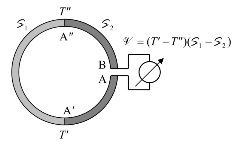
Integrating Equation (\ref{102}) around the loop from point \(A\) to point \(B\), and neglecting the temperature drop across the voltmeter, we get the following simple expression for the thermally-induced difference of the electrochemical potential, usually called either the thermoelectric power or the “thermo e.m.f.”:

\[\begin{align} \mathscr{V} & \equiv \frac{\mu_B '}{q} - \frac{\mu_A'}{q} = \frac{1}{q} \int^B_A \nabla \mu ' \cdot d \mathbf{r} = - \int^B_A \mathcal{S} \nabla T \cdot d\mathbf{r} = -\mathcal{S}_1 \int^{A''}_{A'} \nabla T \cdot d \mathbf{r} - \mathcal{S}_2 \left(\int^{A'}_A \nabla T \cdot d \mathbf{r} + \int^B_{A''} \nabla T \cdot d\mathbf{r} \right) \nonumber \\ & = -\mathcal{S}_1 (T''-T' ) - \mathcal{S}_2 (T' - T'' ) \equiv (\mathcal{S}_1 - \mathcal{S}_2) (T'-T''). \label{103} \end{align}\]

(Note that according to Equation (\ref{103}), any attempt to measure such voltage across any two points of a uniform conductor would give results depending on the voltmeter wire materials, due to an unintentional gradient of temperature in them.)

Using thermocouples is a very popular, inexpensive method of temperature measurement – especially in the few-hundred-\(^{\circ}\)C range where gas- and fluid-based thermometers are not too practicable, if a 1\(^{\circ}\)C-scale accuracy is sufficient. The temperature responsivity (\(\mathcal{S}_1 – \mathcal{S}_2\)) of a typical popular thermocouple, chromel-constantan,⁶³ is about \(70 \mu V/\)\(^{\circ}\)C. To understand why the typical values of \(\mathcal{S}\) are so small, let us discuss the Seebeck effect's physics. Superficially, it is very simple: particles, heated by an external source, diffuse from it toward the colder parts of the conductor, carrying electrical current with them if they are electrically charged. However, this naïve argument neglects the fact that at \(\mathbf{j} = 0\), there is no total flow of particles. For a more accurate interpretation, note that inside the integral (\ref{98}), the Seebeck effect is described by the factor \((\varepsilon – \mu )/T\), which changes its sign at the Fermi surface, i.e. at the same energy where the term \([-\partial \langle N(\varepsilon )\rangle /\partial \varepsilon ]\), describing the availability of quantum states for transport (due to their intermediate occupancy \(0 < \langle N(\varepsilon )\rangle < 1)\), reaches its peak. The only reason why that integral does not vanish completely, and hence \(\mathcal{S} \neq 0\), is the growth of the first factor under the integral (which describes the density of available quantum states on the energy scale) with \(\varepsilon \), so the hotter particles (with \(\varepsilon > \mu \)) are more numerous and hence carry more heat than the colder ones.

The Seebeck effect is not the only result of a temperature gradient; the same diffusion of particles also causes the less subtle effect of heat flow from the region of higher \(T\) to that with lower \(T\), i.e. the effect of thermal conductivity, well known from our everyday practice. The density of this flow (i.e. that of thermal energy) may be calculated similarly to that of the electric current – see Equation (\(6.2.8\)), with the natural replacement of the electric charge \(q\) of each particle with its thermal energy \((\varepsilon – \mu )\):

\[\mathbf{j}_h = \int (\varepsilon - \mu ) \mathbf{v} w d^3 p. \label{104}\]

(Indeed, we may look at this expression is as at the difference between the total energy flow density, \(\mathbf{j}_{\varepsilon} = \int \varepsilon \mathbf{v}wd^3p\), and the product of the average energy needed to add a particle to the system \((\mu )\) by the particle flow density, \(\mathbf{j}_n = \int \mathbf{v}wd^3p \equiv \mathbf{j}/q\).)⁶⁴ Again, at equilibrium \((w = w_0)\) the heat flow vanishes, so that \(w\) in Equation (\ref{104}) may be replaced with its perturbation \(\tilde{w}\), which already has been calculated – see Equation (\ref{96}). The substitution of that expression into Equation (\ref{104}), and its transformation exactly similar to the one performed above for the electric current \(\mathbf{j}\), yields

\[\mathbf{j}_h = \sigma \Pi \left( - \frac{\nabla \mu '}{q} \right) + \kappa (- \nabla T ), \label{105}\]

with the coefficients \(\Pi\) and \(\kappa\) given, in our approximation, by the following formulas:

Peltier coefficient:

\[\boxed{\sigma \Pi = \frac{gq\tau}{(2\pi \hbar )^3} \frac{4\pi}{3} \int^{\infty}_0 (8m\varepsilon^3)^{1/2} (\varepsilon - \mu) \left[ - \frac{\partial \langle N(\varepsilon ) \rangle}{\partial \varepsilon } \right] d\varepsilon , } \label{106}\]

Thermal conductivity:

\[\boxed{\kappa = \frac{g\tau}{(2\pi \hbar )^3} \frac{4\pi}{3} \int^{\infty}_0 (8m\varepsilon^3)^{1/2} \frac{(\varepsilon - \mu)^2}{T} \left[ - \frac{\partial \langle N(\varepsilon ) \rangle}{\partial \varepsilon } \right] d\varepsilon . } \label{107}\]

Besides the missing factor \(T\) in the denominator, the integral in Equation (\ref{106}) is the same as the one in Equation (\ref{98}), so that the constant \(\Pi\) (called the Peltier coefficient ⁶⁵), is simply and fundamentally related to the Seebeck coefficient:

\(\Pi\) vs. \(\mathcal{S}\):

\[\boxed{\Pi = \mathcal{S}T . }\label{108}\]

On the other hand, the integral in Equation (\ref{107}) is different, but may be readily calculated, for the most important case of a degenerate Fermi gas, using the Sommerfeld expansion in the form (\ref{99}), with \(f(\varepsilon ) \equiv (8m\varepsilon^3)^{1/2}(\varepsilon – \mu )^2/T\), for which \(f(\mu ) = 0\) and \(d^2f/d\varepsilon^2|_{\varepsilon =\mu} = 2(8m\mu^3)^{1/2}/T \approx 2(8m\varepsilon F^3)^{1/2}/T\), so that

\[\kappa = \frac{g\tau}{(2\pi \hbar )^3} \frac{4\pi}{3} \frac{\pi^2}{6} T^2 \frac{2(8m\varepsilon^3_F)^{1/2}}{T} \equiv \frac{\pi^2}{3} \frac{n\tau T}{m} . \label{109}\]

Comparing the result with Equation (\(6.2.14\)), we get the so-called Wiedemann-Franz law ⁶⁷

Wiedemann-Franz law:

\[\boxed{ \frac{\kappa}{\sigma} = \frac{\pi^2}{3}\frac{T}{q^2}.}\label{110}\]

This relation between the electric conductivity \(\sigma\) and the thermal conductivity \(\kappa\) is more general than our formal derivation might imply. Indeed, it may be shown that the Wiedemann-Franz law is also valid for an arbitrary anisotropy (i.e. an arbitrary Fermi surface shape) and, moreover, well beyond the relaxation-time approximation. (For example, it is also valid for the scattering integral (\(6.1.12\)) with an arbitrary angular dependence of rate \(\Gamma \), provided that the scattering is elastic.) Experiments show that the law is well obeyed by most metals, but only at relatively low temperatures, when the thermal conductance due to electrons is well above the one due to lattice vibrations, i.e. phonons – see Sec. 2.6. Moreover, for a non-degenerate gas, Equation (\ref{107}) should be treated with the utmost care, in the context of the definition (\ref{105}) of this coefficient \(\kappa \). (Let me leave this issue for the reader's analysis.)

Now let us discuss the effects described by Equation (\ref{105}), starting from the less obvious, first term on its right-hand side. It describes the so-called Peltier effect, which may be measured in the loop geometry similar to that shown in Figure \(\PageIndex{1}\), but now driven by an external voltage source – see Figure \(\PageIndex{2}\).

Figure \(\PageIndex{2}\): The Peltier effect at \(T =\) const.

The voltage drives a certain dc current \(I = jA\) (where \(A\) is the area of conductor's cross-section), necessarily the same in the whole loop. However, according to Equation (\ref{105}), if materials 1 and 2 are different, the power \(\mathscr{P} = j_hA\) of the associated heat flow is different in two parts of the loop.⁶⁸ Indeed, if the whole system is kept at the same temperature \((\nabla T = 0)\), the integration of that relation over the cross-sections of each part yields

\[\mathscr{P}_{1,2} = \Pi_{1,2} A_{1,2} \sigma_{1,2} \left(-\frac{\nabla \mu '}{q}\right)_{1,2} = \Pi_{1,2} A_{1,2}j_{1,2} = \Pi_{1,2}I_{1,2} = \Pi_{1,2}I, \label{111}\]

where, at the second step, Equation (\(6.3.6\)) for the electric current density has been used. This equality means that to sustain a constant temperature, the following power difference,

Peltier effect:

\[\boxed{\Delta \mathscr{P} = (\Pi_1 - \Pi_2 )I, } \label{112}\]

has to be extracted from one junction of the two materials (in Figure \(\PageIndex{2}\), shown on the top), and inserted into the counterpart junction.

If a constant temperature is not maintained, the former junction is heated (in excess of the bulk, Joule heating), while the latter one is cooled, thus implementing a thermoelectric heat pump/refrigerator. Such Peltier refrigerators, which require neither moving parts nor fluids, are very convenient for modest (by a few tens \(^{\circ}\)C) cooling of relatively small components of various systems – from sensitive radiation detectors on mobile platforms (including spacecraft), all the way to cold drinks in vending machines. It is straightforward to use the above formulas to show that the practical efficiency of active materials used in such thermoelectric refrigerators may be characterized by the following dimensionless figure-of-merit,

\[\text{ZT} \equiv \frac{\sigma \mathcal{S}^2}{\kappa}T. \label{113}\]

Finally, let us discuss the second term of Equation (\ref{105}), in the absence of \(\nabla \mu '\) (and hence of the electric current) giving

Fourier law:

\[ \boxed{ \mathbf{j}_h = −\kappa \nabla T ,} \label{114}\]

This equality should be familiar to the reader because it describes the very common effect of thermal conductivity. Indeed, this linear relation is much more general than the particular expression (\ref{107}) for \(\kappa \): for sufficiently small temperature gradients it is valid for virtually any medium – for example, for insulators. (The left column in Table \(\PageIndex{1}\) gives typical values of \(\kappa\) for most common and/or representative materials.) Due to its universality and importance, Equation (\ref{114}) has deserved its own name – the Fourier law.⁷⁰

Acting absolutely similarly to the derivation of other continuity equations, such as Eqs. (\(5.6.12-5.6.13\)) for the classical probability, and Equation (\(6.3.14\)) for the electric charge,⁷¹ let us consider the conservation of the aggregate variable corresponding to \(\mathbf{j}_h\) – the internal energy \(E\) within a time-independent volume \(V\). According to the basic Equation (\(1.3.5\)), in the absence of media's expansion (\(dV = 0\) and hence \(d\mathscr{W} = 0\)), the energy change⁷² has only the thermal component, so its only cause may be the heat flow through its boundary surface \(S\):

\[\frac{dE}{dt} = - \oint_S \mathbf{j}_h \cdot d^2 \mathbf{r}. \label{115}\]

\[E = C_V T = \int_V c_V T d^3 r, \label{116}\]

where \(c_V\) is the volumic specific heat, i.e. the heat capacity per unit volume (see the right column in Table \(\PageIndex{1}\)).

Table \(\PageIndex{1}\): Approximate values of two major thermal coefficients of some materials at 20\(^{\circ}\)C.

Material	\(\kappa (W\cdot m^{-1}\cdot K^{-1})\)	\(c_V (J\cdot K^{-1}\cdot m^{-3})\)
Air^(a),(b)	0.026	\(1.2 \times 10^3\)
Teflon (\([\ce{C2F4}]_n\))	0.25	\(0.6 \times 10^6\)
Water^(b)	0.60	\(4.2 \times 10^6\)
Amorphous silicon dioxide	1.1-1.4	\(1.5 \times 10^6\)
Undoped silicon	150	\(1.6 \times 10^6\)
Aluminum^(c)	235	\(2.4 \times 10^6\)
Copper\(^{(c)}\)	400	\(3.4 \times 10^6\)
Diamond	2,200	\(1.8 \times 10^6\)

^(a)At ambient pressure.

^(b)In fluids (gases and liquids), heat flow may be much enhanced by temperature-gradient-induced turbulent circulation – convection, which is highly dependent on the system's geometry. The given values correspond to conditions preventing the convection.

^(c)In the context of the Wiedemann-Franz law (valid for metals only!), the values of \(\kappa\) for Al and Cu correspond to the Lorenz numbers, respectively, \(2.22 \times 10^{-8} W\cdot \Omega \cdot K^{-2}\) and \(2.39 \times 10^{-8} W\cdot \Omega \cdot K^{-2}\), in a pretty impressive comparison with the universal theoretical value of \(2.45 \times 10^{-8}W\cdot \Omega \cdot K^{-2}\) given by Equation (\ref{110}).

Now applying to the right-hand side of Equation (\ref{115}) the divergence theorem,⁷⁴ and taking into account that for a time-independent volume the full and partial derivatives over time are equivalent, we get

\[\int_V \left( c_V \frac{\partial T}{\partial t} + \nabla \cdot \mathbf{j}_h \right) d^3 r = 0, \label{117}\]

This equality should hold for any time-independent volume \(V\), which is possible only if the function under the integral equals zero at any point. Using Equation (\ref{114}), we get the following partial differential equation, called the heat conduction equation (or, rather inappropriately, the “heat equation”):

Heat conduction equation:

\[\boxed{ c_V (\mathbf{r}) \frac{\partial T}{\partial t} - \nabla \cdot [\kappa(\mathbf{r}) \nabla T ] = 0, } \label{118}\]

where the spatial arguments of the coefficients \(c_V\) and \(\kappa\) are spelled out to emphasize that this equation is valid even for nonuniform media. (Note, however, that Equation (\ref{114}) and hence Equation (\ref{118}) are valid only if the medium is isotropic.)

In a uniform medium, the thermal conductivity \(\kappa\) may be taken out from the external spatial differentiation, and the heat conduction equation becomes mathematically similar to the diffusion equation (\(5.6.11\)), and also to the drift-diffusion equation (\(6.3.15\)) in the absence of drift (\(\nabla U = 0\)):

\[\frac{\partial T}{\partial t} = D_T \nabla^2 T, \quad \text{ with } D_T \equiv \frac{\kappa}{c_V}. \label{119}\]

This means, in particular, that the solutions of these equations, discussed earlier in this course (such as Eqs. (\(5.6.7\))-(\(5.6.8\)) for the evolution of the delta-functional initial perturbation) are valid for Equation (\ref{119}) as well, with the only replacement \(D \rightarrow D_T\). This is why I will leave a few other examples of the solution of this equation for the reader's exercise.

Let me finish this chapter (and this course as a whole) by emphasizing again that due to time/space restrictions I was able to barely scratch the surface of physical kinetics.⁷⁵