
3.2: Motion with Constant Acceleration
- Page ID
- 19373
Until now, we have considered motion where the velocity is a constant (i.e. where velocity does not change with time). Suppose that we wish to describe the position of a falling object that we released from rest at time \(t=0\text{s}\). The object will start with a velocity of 0 m/s and it will accelerate as it falls. We say that an object is “accelerating” if its velocity is not constant. As we will see in later chapters, objects that fall near the surface of the Earth experience a constant acceleration (their velocity changes at a constant rate).
Formally, we define acceleration as the rate of change of velocity. Recall that velocity is the rate of change of position, so acceleration is to velocity what velocity is to position. In particular, we saw that if the velocity, \(v_{x}\), is constant, then position as a function of time is given by:
\[x(t) = x_{0} + v_{x}t\]
In analogy, if the acceleration is constant, then the velocity as a function of time is given by:
\[v_{x}(t) = v_{0x} + a_{x}t\]
where \(a_{x}\) is the “acceleration” and \(v_{0x}\) is the velocity of the object at \(t=0\). We can work out the dimensions of acceleration for this equation to make sense. Since we are adding \(v_{0x}\) and \(a_{x}t\), we need the dimensions of \(a_{x}t\) to be velocity:
\(\begin{aligned} \left[a_{x}t\right]&=\frac{L}{T} \\[4pt] \left[a_{x}\right]&=\frac{L}{T^{2}} \end{aligned}\)
Acceleration thus has dimensions of length over time squared, with corresponding S.I. units of \(\text{m/s}^{2}\) (meters per second squared or meters per second per second). In order to describe the position of an object that is accelerating, we cannot use Equation 3.2.1, since it is only correct if the velocity is constant.
In Section 3.3 Using calculus to obtain acceleration from position, we will show that the position as a function of time, \(x(t)\), of an object with constant acceleration, \(a_{x}\), is given by:
\[x(t)=x_{0}+v_{0x}t+\frac{1}{2}a_{x}t^{2}\]
where, at \(t = 0\), the object was at position \(x = x_{0}\) and had a velocity \(v_{0x}\).
A ball is thrown upwards with a velocity of \(10\text{m/s}\). After what distance will the ball stop before falling back down? Assume that gravity causes a constant downwards acceleration of \(9.8\text{m/s}^{2}\).
Solution
We will solve this problem in the following steps:
- Setup a coordinate system (define the \(x\)-axis).
- Identify the condition that corresponds to the ball stopping its upwards motion and falling back down.
- Determine the distance at which the ball stopped.
Since we throw the ball upwards with an initial velocity upwards, it makes sense to choose an \(x\)-axis that points up and has the origin at the point where we release the ball. With this choice, referring to the variables in Equation 3.2.3, we have:
\(\begin{aligned} x_{0}&=0 \\[4pt] v_{0x}&=+10\text{m/s} \\[4pt] a_{x}&=-9.8\text{m/s}^{2} \end{aligned}\)
where the initial velocity is in the positive x-direction, and the acceleration, \(a_{x}\), is in the negative direction (the velocity will be getting smaller and smaller, so its rate of change is negative).
The condition for the ball to stop at the top of the trajectory is that its velocity will be zero (that is what it means to stop). We can use Equation 3.2.2 to find what time that corresponds to:
\(\begin{aligned} v(t)&=v_{0x}+a_{x}t \\[4pt] 0&=(10\text{m/s})+(-9.8\text{m/s}^{2})t \\[4pt] \therefore t&=\frac{(10\text{m/s})}{(9.8\text{m/s}^{2})}=1.02\text{s} \end{aligned}\)
Now that we know that it took \(1.02\text{s}\) to reach the top of the trajectory, we can find how much distance was covered:
\(\begin{aligned} x(t)&=x_{0}+v_{0x}t+\frac{1}{2}a_{x}t^{2} \\[4pt] x&=(0\text{m})+(10\text{m/s})(1.02\text{s})+\frac{1}{2}(-9.8\text{m/s}^{2})(1.02\text{s})^{2}=5.10\text{m} \end{aligned}\)
and we find that the ball will rise by \(5.10\text{m}\) before falling back down.
Visualizing motion with constant acceleration
When an object has a constant acceleration, its velocity and position as a function of time are described by the two following equations:
\(\begin{aligned} v(t)&=v_{0x}+a_{x}t \\[4pt] x(t)&=x_{0}+v_{0x}t + \frac{1}{2}a_{x}t^{2} \end{aligned}\)
where the velocity changes linearly with time, and the position changes quadratically with time (it goes as \(t^{2}\)). Figure \(\PageIndex{1}\) shows the position and the speed as a function of time for the ball from Example 3.2.1 for the first three seconds of the motion.
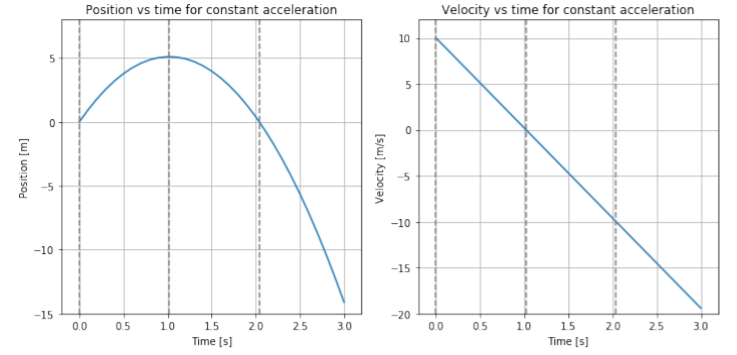
We can divide the motion into three parts (shown by the vertical dashed lines in Figure \(\PageIndex{1}\)):
1) Between \(t=0\text{s}\) and \(t=1.02\text{s}\)
At time \(t=0\text{s}\), the ball starts at a position of \(x=0\text{m}\) (left panel) and has a velocity of \(v_{0x}=10\text{m/s}\) (right panel). During the first second of motion, the position, \((t)\), increases (the ball is moving up), until the position stops increasing at \(t=1.02\text{s}\), as found in Example 3.2.1. During that time, the velocity decreases linearly from \(10\text{m/s}\) to \(0\text{m/s}\) due to the constant negative acceleration from gravity. At \(t=1.02\text{s}\), the velocity is instantaneously \(0\text{m/s}\) and the ball is momentarily at rest (as it reaches the top of the trajectory before falling back down).
2) Between \(t=1.02\text{s}\) and \(t=2.04\text{s}\)
At \(t=1.02\text{s}\), the velocity continues to decrease linearly (it becomes more and more negative) as the ball start to fall back down faster and faster. The position also starts decreasing just after \(t=1.02\text{s}\), as the ball returns back down to the point of release. At \(t=2.04\text{s}\), the ball returns to the point from which it was thrown, and the ball is going with the same velocity \((10\text{m/s})\) as when it was released, but the velocity is negative (downwards motion).
3) After \(t=2.04\text{s}\)
If nothing is there to stop the ball, it continues to move downwards with ever increasing velocity. The position continues to become more negative and the velocity continues to become larger in magnitude and more negative.
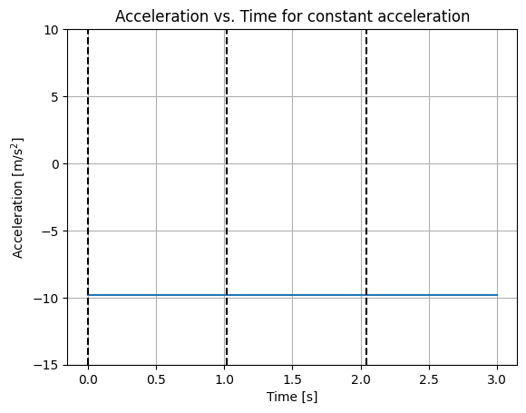
Make a sketch of the acceleration as a function of time corresponding to the position and velocity shown in Figure \(\PageIndex{1}\).
- Answer
- The slope (or derivative) of the velocity vs. time graph is negative and constant. These graphs correspond to the example above where \(a = -9.8 \rm{m/s^2}\).
Speed versus velocity
In the previous example, our language was not quite as precise as it should be when conducting science. Specifically, we need a way to distinguish the situation when the velocity is decreasing (becoming more negative), while the object is actually going faster and faster (after \(t=1.02\text{s}\)). We will use the term speed to refer to how fast an object is moving (how much distance it covers per unit time), and we will use the term velocity to also indicate the direction of the motion. In other words, the speed is the absolute value of the velocity. The speed is thus always positive, whereas the velocity can also be negative.
With this vocabulary, the speed of the ball decreases between \(t=0\text{s}\) and \(t=1.02\text{s}\), and increases thereafter. On the other hand, the velocity continuously decreases (it is always becoming more and more negative). Velocity is thus the more general term since it tells us both the speed and the direction of the motion.