
3.3: Using Calculus to Describe Motion
- Page ID
- 19374
Objects do not necessarily have a constant velocity or acceleration. We thus need to extend our description of the position and velocity of an object to a more general case. This can be done in much the same way as we introduced accelerated motion; namely by pretending that during a very small interval in time, \(∆t\), the velocity and acceleration are constant, and then considering the motion as the sum over many small intervals in time. In the limit that \(∆t\) tends to zero, this will be an accurate description.
Instantaneous and average velocity
Suppose that an object is moving with a non constant velocity, and covers a distance \(\Delta x\) in an amount of time \(\Delta t\). We can define an average velocity, \(v^{avg}\):
\[v^{avg}= \frac{\Delta x}{\Delta t}\]
That is, regardless of our choice of time interval, \(\Delta t\), we can always calculate the average velocity, \(v^{avg}\), of an object over a particular distance. That average velocity will be an average over the interval, between some time \(t\) and \(t+\Delta t\). If we shrink the length of the time interval used to measure the velocity, and take the limit \(\Delta t\rightarrow 0\), we can define the instantaneous velocity:
\[v = \lim_{\Delta t\to 0} \frac{\Delta x}{\Delta t}\]
The instantaneous velocity is the velocity only in that small instant in time where we choose \(\Delta x\) and \(\Delta t\). Another way to read this equation is that the velocity, \(v\), is the slope of the graph of \(x(t)\). Recall that the slope is the “rise over run”, in other words the change in \(x\) divided by the corresponding change in \(t\). Indeed, when we had no acceleration, the position as a function of time, Equation 3.1.1, explicitly had the velocity as the slope of a linear function:
\[x(t) = v_{0x}+v_{x}t\]
If we go back to Figure \(\PageIndex{1}\), where velocity was no longer constant, we can indeed see that the graph of the velocity versus time (\(v(t)\)) corresponds to the instantaneous slope of the graph of position versus time (\(x(t)\)). For \(t<1.02\text{s}\), the slope of the \(x(t)\) graph is positive but decreasing (as is \(v(t)\)). At \(t=1.02\text{s}\), the slope of \(x(t)\) is instantaneously \(0\text{m/s}\) (as is the velocity). Finally, for \(t>1.02\text{s}\), the slope of \(x(t)\) is negative and increasing in magnitude, as is \(v(t)\).
Leibniz and Newton were the first to develop mathematical tools to deal with calculations that involve quantities that tend to zero, as we have here for our time interval \(\Delta t\). Nowadays, we call that field of mathematics “calculus”, and we will make use of it here. Using the vocabulary of calculus, rather than saying that “instantaneous velocity is the slope of the graph of position versus time at some point in time”, we say that “instantaneous velocity is the time derivative of position as a function of time”. We also use a slightly different notation so that we do not have to write the limit \(\lim_{\Delta t\to 0}\):
\[ v(t)=\lim_{\Delta t\to 0} \frac{\Delta x}{\Delta t}=\frac{dx}{dt}=\frac{d}{dt} x(t)\]
where we can really think of \(dt\) as \(\lim_{\Delta t\to 0}\Delta t\), and \(dx\) as the corresponding change in position over an infinitesimally small time interval \(dt\).
Similarly, we introduce the instantaneous acceleration, as the time derivative of \(v(t)\):
\[a_x(t)=\frac{dv}{dt}=\frac{d}{dt}v(t)\]
When looking at a graph of position versus time, it is sometimes hard to tell at first glance whether the speed of the object is increasing or decreasing. This section gives us an easy way to figure it out. The velocity is the instantaneous slope of the graph \(x(t)\), so the speed is the “steepness” of that graph. Simply draw a few lines that are tangent to (meaning just touching) the curve, and see what happens as time increases. If the lines get steeper, the object is speeding up. If they are getting flatter, the object is slowing down.
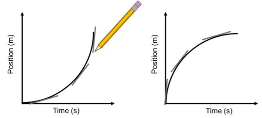
From here, you can also figure out what the direction of the acceleration is. If an object is speeding up, the acceleration and velocity must be in the same direction (i.e. both positive or both negative). If the object is slowing down, they must be in opposite directions. Imagine the graphs in Figure \(\PageIndex{1}\) are describing the motion of a person running in heavy wind. In the graph on the left, the person is running with the wind and accelerating (\(v(t)\) and \(a(t)\) positive), and in the second graph the person is running against the wind and decelerating (\(v(t)\) positive and \(a(t)\) negative).
Using calculus to obtain acceleration from position
Suppose that we know the function for position as a function of time, and that it is given by our previous result (for the case when the acceleration \(a_{x}\) is constant):
\[x(t)=x_0+v_{0x}t+\frac{1}{2}a_{x}t^{2}\]
With our calculus-based definitions above, we should be able to recover that:
\[\begin{aligned} v(t) = v_{0x}t+at\\[4pt] a_x(t) = a_x\end{aligned}\]
Let us start by determining \(v(t)\):
\[\begin{aligned} v(t) = \frac{dx}{dt}=\lim_{\Delta t\to 0} \frac{\Delta x}{\Delta t}\end{aligned}\]
Knowing our function \(x(t)\), we can can rewrite this as:
\[\begin{aligned} \frac{dx}{dt}=\lim_{\Delta t\to 0} \frac{x(t+\Delta t)-x(t)}{\Delta t} \end{aligned}\]
which is the formal definition of the derivative \(\frac{dx}{dt}\) and gives us a prescription to evaluate it. We will proceed as illustrated in Figure \(\PageIndex{1}\):
- Use \(x(t)\) to determine \(\Delta x\) for a small interval \(\Delta t\)
- Divide \(\Delta x\) by \(\Delta t\)
- Take the limit, \(\lim_{\Delta t\to 0}\)
To obtain \(\Delta x\), we introduce a start time, \(t_1\), and an end time \(t_2\) for our time interval, such that \(t_2-t_1=\Delta t\), centerd about a time \(t\). The change in position is then given by:
\[\begin{aligned} \Delta x &= x(t_2) - x(t_1)\\[4pt] &=\left(x_0+v_{0x}t_2+\frac{1}{2}a_xt_2^2\right )- \left(x_0+v_{0x}t_1+\frac{1}{2}a_xt_1^2\right )\\[4pt] &=v_{0x}(t_2-t_1)+\frac{1}{2}a_x(t_2^2-t_1^2)\\[4pt] &=v_{0x}\Delta t+\frac{1}{2}a_x(t_2-t_1)(t_2+t_1)\\[4pt] &=v_{0x}\Delta t+\frac{1}{2}a_x\Delta t (t_2+t_1)\\[4pt]\end{aligned}\]
which we divide by \(\Delta t\) to get \(v(t)\):
\[\begin{aligned} v(t) &= \frac{\Delta x}{\Delta t}\\[4pt] &=\frac{v_{0x}\Delta t+\frac{1}{2}a_x\Delta t (t_2+t_1)}{\Delta t}\\[4pt] &=v_{0x}+\frac{1}{2}a_x(t_2+t_1)\end{aligned}\]
We now take the limit where \(\Delta t\to 0\), namely when \(t_2-t_1\) is very small. As we make the interval small, \(t_2\) and \(t_1\) will both approach the same value of time, say \(t\), corresponding to the time at the center of the interval. In particular, the average of \(t_1\) and \(t_2\), given by \(\frac{1}{2}(t_1+t_2)\), will approach the time at the center of the interval, \(t\). We thus recover the equation for instantaneous velocity:
\[\begin{aligned} v(t) &= v_{0x}+a_xt\end{aligned}\]
Of course, once you become more familiar with calculus, you will be able to directly use the formulas for derivatives to recover the answer:
\[\begin{aligned} v(t) &= \frac{d}{dt}\left( x_0+v_{0x}t+\frac{1}{2}a_xt^2 \right) \\[4pt] &= v_{0x}+at \end{aligned}\]
Similarly, we can now confirm that the acceleration is a constant, independent of time:
\[\begin{aligned} a_x(t) &= \frac{dv}{dt} = \frac{d}{dt}\left(v_{0x}+a_xt \right)\\[4pt] &=a_x\end{aligned}\]
You can easily verify that you obtain this result by first calculating \(v(t)\) at two different times, \(t_1\) and \(t_2\), taking the difference, \(\Delta v = v(t_2)-v(t_1)\), and then taking the limit of \(\lim_{\Delta t\to 0}\frac{\Delta v}{\Delta t}\) to get \(a_x(t)\).
Chloë has been working on a detailed study of how vicuñas run, and found that their position as a function of time when they start running is well modelled by the function \(x(t)=(40\text{m/s}^{2})t^{2}+(20\text{m/s}^{3})t^{3}\). What is the acceleration of the vicuñas?
- \(a_x(t)=40\text{m/s}^{2}\)
- \(a_x(t)=80\text{m/s}^{2}\)
- \(a_x(t)=40\text{m/s}^{2}+(20\text{m/s}^{3})t\)
- \(a_x(t)=80\text{m/s}^{2}+(120\text{m/s}^{3})t\)
"Never heard of vicuñas? Internet!
- Answer
- The acceleration is time dependent. It begins as twice the first term because position depends on \(0.5 a\). Over time, the acceleration changes by \(2\times 3 \times 20 t\), where the three is similar to the factor of 2 in constant acceleration. Therefore, the correct answer is \(a_x(t)=80\text{m/s}^{2}+(120\text{m/s}^{3})t\).
Using calculus to obtain position from acceleration
Now that we saw that we can use derivatives to determine acceleration from position, we will see how to do the reverse and use acceleration to determine position. Let us suppose that we have a constant acceleration, \(a_{x}(t)=a_{x}\), and that we know that at time \(t=0\text{s}\), the object had a speed of \(v_{0x}\) and was located at a position \(x_{0}\).
Since we only know the acceleration as a function of time, we first need to find the velocity as a function of time. We start with:
\[a_{x}(t)=a_{x}=\frac{d}{dt} v(t)\]
which tells us that we know the slope (derivative) of the function \(v(t)\), but not the actual function. In this case, we must do the opposite of taking the derivative, which in calculus is called taking the “anti-derivative” with respect to \(t\) and has the symbol \(\int dt\). In other words, if:
\[\frac{d}{dt} v(t) =a_{x}(t)\]
then:
\[v(t) =\int a_{x}(t) dt +C\]
where as we will see later, the constant \(C\) is required in order for the function \(v(t)\) to go through the point \(v(t=0)=v_{0x}\). All we need now is to determine how to calculate the anti-derivative, \(\int a_{x}(t) dt\). Since in this case, \(a_{x}(t)\) is a constant, \(a_{x}\), we can determine the anti-derivative quite easily.
For a small interval in time, \(\Delta t\), the velocity will change by a small amount, \(\Delta v\), such that:
\[\begin{aligned} a_x &= \frac{\Delta v}{\Delta t}\\[4pt] \Delta v &= a_x \Delta t\end{aligned}\]
If we label the start time of the interval as \(t_1\) and the end of the interval as \(t_2\), we have:
\[\begin{aligned} \Delta t &= t_2 - t_1 \\[4pt] \Delta v &= v(t_2) - v(t_1) = a_x \Delta t\\[4pt] \therefore v(t_2) &= v(t_1)+a_x\Delta t\end{aligned}\]
If we set \(t_1=0\text{s}\) to correspond to the point where \(v(t)=v_{0x}\), then we can write the velocity at \(t_2\) as:
\[\begin{aligned} v(t_2) = v(t=\Delta t) = v_{0x}+a_x\Delta t\end{aligned}\]
and we see that the velocity changed by an amount \(a \Delta t\) over a period of time \(\Delta t\). Since \(a_x\) is the same at all times, this is always true, and after a period of time \(t = N\Delta t\), the velocity will have changed by \(N a_x \Delta t\), and we recover the original equation for velocity as a function of time when acceleration is constant:
\[\begin{aligned} v(t=N \Delta t) &= v_{0x}+Na_x\Delta t\\[4pt] \therefore v(t) &= v_{0x}+a_xt\\[4pt]\end{aligned}\]
We can identify the anti-derivative for the case where \(a(t)\) is constant:
\[\begin{aligned} \frac{d}{dt} v(t) &=a_x\\[4pt] \int a_x dt &=a_xt +C\end{aligned}\]
where the constant, \(C\), is given by \(v_{0x}\).
\[v(t)=C+a_{x}t=v_{0x}+a_{x}t\]
and we recover the formula for velocity when the acceleration is constant. Now that we know the velocity as a function of time, we can take one more anti-derivative with respect to time to obtain the position:
\(\begin{aligned}&v(t)=\frac{dx}{dt} \\[4pt] &\therefore x(t)=\int v(t)dt\end{aligned}\)
In the case where acceleration is constant, this gives:
\(\begin{aligned} x(t)&=\int v(t)dt \\[4pt] &=\int (v_{0x}+a_{x}t)dt \\[4pt] &=v_{0x}t+\frac{1}{2}a_{x}t^{2}+C' \end{aligned}\)
where \(C'\) is a different constant than the one we had when determining velocity. The constant is given by our initial conditions. If the object was located at position \(x = x_{0}\) at time \(t = 0\), then \(C'= x_{0}\) and we recover the equation for position as a function of time for constant acceleration:
\[x(t)=x_{0}+v_{0x}t+\frac{1}{2}a_{x}t^{2}\]
To now obtain position as a function of time, we proceed in the same manner, namely:
- Define a small interval in time \(\Delta t\)
- Calculate the corresponding change in position \(\Delta x\)
- Add \(\Delta x\) to our original position, and repeat.
Again, we have the time-derivative of the position equal to a function of time:
\[\begin{aligned} \frac{d}{dt}x(t)=v(t)=v_{0x}+a_xt\end{aligned}\]
and we need to find the anti-derivative:
\[\begin{aligned} x(t) = \int \left( v_{0x}+av_xt \right) dt \end{aligned}\]
given that, at time \(t=0\), the position was \(x=x_0\). After a small interval in time, \(\Delta t\), the position will have changed by an amount \(\Delta x\):
\[\begin{aligned} \Delta x &= v(t) \Delta t\\[4pt]\end{aligned}\]
so that the position at time \(t=\Delta t\) will be given by:
\[\begin{aligned} x(t=\Delta t) &= x_0+ \Delta x\\[4pt] & = x_0+v(t) \Delta t\end{aligned}\]
The problem here is to evaluate \(v(t)\) since the velocity changes throughout the interval. One possible choice is to evaluate the velocity at \(t = \frac{1}{2}\Delta t\), midway in the interval, as we did before. We could also choose to use the velocity at the beginning or at the end of the time interval, as all three choices will converge to the same value when \(\Delta t \to 0\). For now, we will leave the choice open and simply call the velocity that we use \(v_1\) to indicate that it is the velocity in the first interval. We thus write the position, \(x(t=\Delta t)\), after a time interval \(\Delta t\) as:
\[\begin{aligned} x(t=\Delta t) = x_0+v_1\Delta t\end{aligned}\]
The position, \(x(t=2\Delta t)\), after another interval in time \(\Delta t\) will then be given by:
\[\begin{aligned} x(t=2\Delta t) &= x(t=\Delta t)+v_2\Delta t\\[4pt] &=x_0+v_1\Delta t+v_2\Delta t\end{aligned}\]
where \(v_2\) is the velocity over the second interval in time (different than \(v_1\), since velocity changes with time). For the Nth interval, we label the position \(x_N=x(t=N\Delta t)\):
\[\begin{aligned} x_N=x(t=N\Delta t)&=x_0+v_1\Delta t+v_2\Delta t+\dots+v_N\Delta t\\[4pt] &=x_0+\sum_{i=1}^Nv_i\Delta t \end{aligned}\]
where we made use of the summation notation (\(\sum\)) to avoid writing out every term. The above equation is only correct in the limit of \(\Delta t\to 0\), in which case it must be the anti-derivative of \(v(t)\):
\[\begin{aligned} x(t) &= \int v(t) dt\\[4pt] &= x_0+\lim_{\Delta t\to 0}\sum_{i=1}^Nv_i\Delta t \end{aligned}\]
so that we can identify:
\[ \int v(t) dt=\lim_{\Delta t\to 0}\sum_{i=1}^Nv_i\Delta t + C \]
where it is understood that \(v_i\) is the “average” velocity in the ith interval, and the constant \(C=x_0\) ensures that \(x(t=0)=x_0\). This is now a general definition for the anti-derivative, as we have made no specific assumption about the function \(v(t)\). Equation 3.3.10 tells us that the anti-derivative of a function (in this case, \(v(t)\)) can be obtained from a sum.
The sum shows the function \(v(t)\) and several intervals \(\Delta t\). Over each interval, \(i\), we labeled the average velocity, \(v_i\). As the intervals shrink, \(\Delta t\to 0\), the average velocity \(v_i\) approaches the instantaneous velocity, \(v(t)\), at the center for the interval. Since the function \(v(t)\) is linear (for constant acceleration), the speed at the middle of an interval is exactly equal to the average speed in the interval. Taking \(v_i\) as the speed in the middle of the interval, we then see that each term in the sum, \(v_i\Delta t\), is equal to the area between the curve \(v(t)\) and the t-axis. This is illustrated for the second term in the sum, \(v_2\Delta t\).
The anti-derivative of a function is thus related to the area between the function and the horizontal axis. If we specify limits on the horizontal axis between which we calculate the area, then the anti-derivative is called an integral. For example, if we wish to calculate the sum of \(v_i \Delta t\) for values between \(t_a\) and \(t_b\), we would write the integral as:
\[ \int_{t_a}^{t_b}v(t) dt = \lim_{\Delta t\to 0}\sum_{i=1}^Nv_i\Delta t \]
where the sum is such that for \(i=1\), \(v_i\) is close to \(v(t=t_a)\) and for \(i=N\), \(v_N\) is close to \(v(t=t_b)\). An illustration of taking the integral of \(v(t)\) is shown where the sum is shown for two different values of \(\Delta t\). It is clear that as \(\Delta t \to 0\), the sum becomes equal to the area between the curve and the horizontal axis.
Since \(v(t)\) is a linear function when acceleration is constant, we can easily calculate the area between the curve and the horizontal axis. In the case of a linear function, \(v(t)=v_{0x}+at\), the area is a trapezoid, and we have:
\[\begin{aligned} \int_{t_a}^{t_b}v(t) dt &= \text{base}\times\text{average height}\\[4pt] &=(t_b-t_a)\times\frac{1}{2}\left(v(t_a)+v(t_b)\right)\\[4pt] &=(t_b-t_a)\frac{1}{2}(v_{0x}+a_xt_a+v_{0x}+a_xt_b)\\[4pt] &=\left( \frac{1}{2}(v_{0x}t_b+a_xt_at_b+v_{0x}t_b+a_xt_b^2) \right)- \left( \frac{1}{2}(v_{0x}t_a+a_xt_a^2+v_{0x}t_a+a_xt_bt_a) \right)\\[4pt] &=\left( v_{0x}t_b+\frac{1}{2}a_xt_b^2 \right)-\left( v_{0x}t_a+\frac{1}{2}a_xt_a^2 \right)\end{aligned}\]
If we define a new function, \(V(t)=v_{0x}t+\frac{1}{2}a_xt^{2}\), then we have:
\[ \int_{t_{a}}^{t_{b}}v(t) dt = V(t_{b}) -V(t_{a})\]
In other words, given a function, \(v(t)\), the integral of that function between two values \(t_a\) and \(t_b\) can be found by evaluating a different function, \(V(t)\), at the end points \(t_a\) and \(t_b\). As you will see in your calculus course, the function \(V(t)\) is precisely what we call the anti-derivative:
\[ \int v(t) dt= V(t) + C\]
which has derivative:
\[\begin{aligned} \frac{dV}{dt}=v(t)\end{aligned}\]
Note that when taking the integral, the constant \(C\) always cancels.
Choose the graph of \(x(t)\) for the case when acceleration is given by \(a(t) = Aω^{2}cos(ωt)\), where \(ω\) and \(A\) are positive constants. The velocity and position are zero at \(t = 0\).
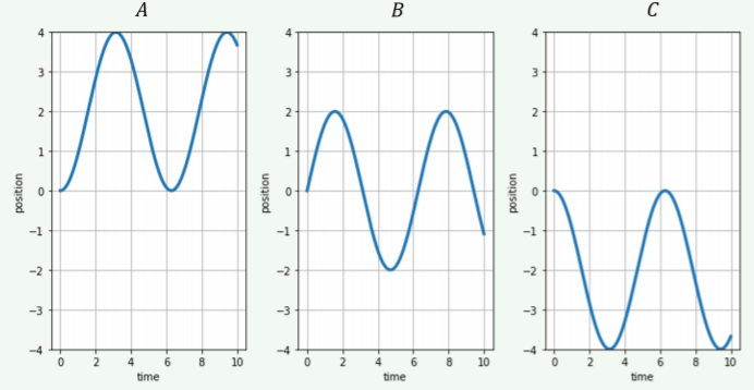
- Figure A
- Figure B
- Figure C
- Answer
- Figure A. The acceleration is positive near \(t=0 \text{s}\) as described by the second derivative, which is concave up.
The acceleration of a cricket jumping sideways is observed to increase linearly with time, that is, \(a_{x}(t)=a_{0}+jt\), where \(a_{0}\) and \(j\) are constants. What can you say about the velocity of the cricket as a function of time?
- it is constant
- it increases linearly with time (\(v(t)\propto t\))
- it increases quadratically with time (\(v(t)\propto t^{2}\))
- it increases with the cube of time (\(v(t)\propto t^{3}\))
- Answer
- C. We know velocity is linear in time (\(v(t)\propto t\)) when \(a\) is constant. If \(a\) becomes linearly time-dependent (\(a(t)\propto t\)), the velocity will change its dependence by the same change in time-dependence (\(v(t)\propto t^{2}\)).