4.1: Motion in two Dimensions

Using vectors to describe motion in two dimensions

We can specify the location of an object with its coordinates, and we can describe any displacement by a vector. First, consider the case of an object moving with a constant velocity in a particular direction. We can specify the position of the object at any time, \(t\), using its position vector, \(\vec r(t)\), which is a function of time. The position vector is a vector that goes from the origin of the coordinate system to the position of the object. We can describe the \(x\) and \(y\) components of the position vector with independent functions, \(x(t)\), and \(y(t)\), that correspond to the \(x\) and \(y\) coordinates of the object at time \(t\), respectively:

\[\begin{aligned} \vec r(t) = \begin{pmatrix} x(t) \\[4pt] y(t) \\[4pt] \end{pmatrix}= x(t) \hat x + y(t) \hat y\end{aligned}\]

Suppose that in a period of time \(\Delta t\), the object goes from a position described by the position vector \(\vec r_1\) to a position described by the position vector \(\vec r_2\), as illustrated in Figure \(\PageIndex{1}\).

Figure \(\PageIndex{1}\): Illustration of a displacement vector, \(∆\stackrel{\rightarrow}{r} = \stackrel{\rightarrow}{r_{2}}−\stackrel{\rightarrow}{r_{1}}\), for an object that was located at position \(\stackrel{\rightarrow}{r_{1}}\) at time \(t_{1}\) and at position \(\stackrel{\rightarrow}{r_{2}}\) at time \(t_{2} = t_{1} + ∆t\).

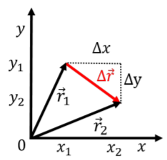
We can define a displacement vector, \(\Delta \vec r=\vec r_2-\vec r_1\), and by analogy to the one dimensional case, we can define an average velocity vector, \(\vec v\) as:

\[ \vec v = \frac{\Delta \vec r}{\Delta t}\]

The average velocity vector will have the same direction as \(\Delta \vec r\), since it is the displacement vector divided by a scalar (\(\Delta t\)). The magnitude of the velocity vector, which we call “speed”, will be proportional to the length of the displacement vector. If the object moves a large distance in a small amount of time, it will thus have a large velocity vector. This definition of the velocity vector thus has the correct intuitive properties (points in the direction of motion, is larger for faster objects).

For example, if the object went from position \((x_1,y_1)\) to position \((x_2,y_2)\) in an amount of time \(\Delta t\), the average velocity vector is given by:

\[\begin{aligned} \vec v &= \frac{\Delta \vec r}{\Delta t}\\[4pt] &=\frac{1}{\Delta t}\begin{pmatrix} x_2-x_1 \\[4pt] y_2-y_1 \\[4pt] \end{pmatrix}\\[4pt] &=\frac{1}{\Delta t}\begin{pmatrix} \Delta x \\[4pt] \Delta y \\[4pt] \end{pmatrix}\\[4pt] \end{aligned}\]

\[\begin{aligned} &=\begin{pmatrix} \frac{\Delta x}{\Delta t} \\[4pt] \frac{\Delta y}{\Delta t}\\[4pt] \end{pmatrix}\\[4pt] &=\begin{pmatrix} v_x \\[4pt] v_y \\[4pt] \end{pmatrix}\\[4pt] \therefore \vec v &= v_x\hat x+v_y\hat y \end{aligned}\]

That is, the \(x\) and \(y\) components of the average velocity vector can be found by separately determining the average velocity in each direction. For example, \(v_x=\frac{\Delta x}{\Delta t}\) corresponds to the average velocity in the \(x\) direction, and can be considered independent from the velocity in the \(y\) direction, \(v_y\). The magnitude of the average velocity vector (i.e. the average speed), is given by:

\[\begin{aligned} ||\vec v||&=\sqrt{v_x^2+v_y^2}=\frac{1}{\Delta t}\sqrt{\Delta x^2+\Delta y^2}=\frac{\Delta r}{\Delta t}\end{aligned}\]

where \(\Delta r\) is the magnitude of the displacement vector. Thus, the average speed is given by the distance covered divided by the time taken to cover that distance, in analogy to the one dimensional case.

Exercise \(\PageIndex{1}\)

A llama runs in a field from a position \((x_1,y_1)=(2\text{m},5\text{m})\) to a position \((x_2,y_2)=(6\text{m},8\text{m})\) in a time \(\Delta t=0.5\text{s}\), as measured by Marcel, a llama farmer standing at the origin of the Cartesian coordinate system. What is the average speed of the llama?

1. \(1\text{ m/s}\)
2. \(5\text{ m/s}\)
3. \(10\text{ m/s}\)
4. \(15\text{ m/s}\)

Answer

C. The llama has an average velocity \((v_{x}, v_y) = (x_2-x_1,y_2-y_1)/\Delta t=(6-2, 8-5)/0.5 = (4, 3)/0.5 = (8, 6)\text{m/s}\). By the Pythagorean Theorem the average speed is \(v = \sqrt{8^2+6^2} = 10 \text{m/s}\).

If the velocity of the object is not constant, then we define the instantaneous velocity vector by taking the limit \(\Delta t\to 0\):

\[\vec v(t) = \lim_{\Delta t \to 0}\frac{\Delta \vec r}{\Delta t}=\frac{d\vec r}{dt}\]

which gives us the time derivative of the position vector (in one dimension, it was the time derivative of position). Writing the components of the position vector as functions \(x(t)\) and \(y(t)\), the instantaneous velocity becomes:

\[\stackrel{\rightarrow}{v}(t)=\frac{d}{dt}\stackrel{\rightarrow}{r}(t)\]

\[\begin{aligned} &=\frac{d}{dt} \begin{pmatrix} x(t) \\[4pt] y(t) \\[4pt] \end{pmatrix}\nonumber\\[4pt] &=\begin{pmatrix} \frac{dx}{dt} \\[4pt] \frac{dy}{dt} \\[4pt] \end{pmatrix}\nonumber\\[4pt] &=\begin{pmatrix} v_x(t) \\[4pt] v_y(t) \\[4pt] \end{pmatrix}\nonumber\\[4pt] \therefore \vec v(t) &= v_x(t)\hat x+v_y(t)\hat y \nonumber \end{aligned}\]

where, again, we find that the components of the velocity vector are simply the velocities in the \(x\) and \(y\) direction. This means that we can treat motion in two dimensions as two times one-dimensional motion: a motion along \(x\) and a separate motion along \(y\). This highlights the usefulness of the vector notation for allowing us to use one vector equation (\(\vec v=\frac{d}{dt}\Delta \vec r\)) to represent two equations (one for \(x\) and one for \(y\)).

Similarly the acceleration vector is given by:

\[\stackrel{\rightarrow}{a}(t)=\frac{d}{dt}\stackrel{\rightarrow}{v}(t) \]

\[\begin{aligned} &=\begin{pmatrix} \frac{dv_x}{dt} \\[4pt] \frac{dv_y}{dt} \\[4pt] \end{pmatrix}\nonumber\\[4pt] &=\begin{pmatrix} a_x(t) \\[4pt] a_y(t) \\[4pt] \end{pmatrix}\nonumber\\[4pt] \therefore \vec a(t) &= a_x(t)\hat x+a_y(t)\hat y \nonumber \end{aligned}\]

If an object is at position \(\vec r_0=(x_0,y_0)\) with a velocity vector \(\vec v_0=v_{0x}\hat x + v_{0y}\hat y\) at time \(t=0\), and has a constant acceleration vector¹, \(\vec a = a_x\hat x+a_y\hat y\), then the velocity vector at some later time \(t\), \(\vec v(t)\), is given by:

\[\begin{aligned} \vec v(t) = \vec v_0 + \vec a t\end{aligned}\]

Or, if we write out the components explicitly:

\[\begin{aligned} \begin{pmatrix} v_x(t) \\[4pt] v_y(t) \\[4pt] \end{pmatrix} = \begin{pmatrix} v_{0x} \\[4pt] v_{0y} \\[4pt] \end{pmatrix} + \begin{pmatrix} a_xt \\[4pt] a_yt \\[4pt] \end{pmatrix}\end{aligned}\]

these be considered as two independent equations for the components of the velocity vector:

\[\begin{aligned} v_x(t)&=v_{0x}+a_xt \\[4pt] v_y(t)&=v_{0y}+a_yt \\[4pt]\end{aligned}\]

which is the same equation that we had for one dimensional kinematics, but once for each coordinate. The position vector is given by:

\[\begin{aligned} \vec r(t) = \vec r_0 + \vec v_0 t + \frac{1}{2} \vec at^2\end{aligned}\]

with components:

\[\begin{aligned} x(t) &= x_0+v_{0x}t+\frac{1}{2}a_xt^2\\[4pt] y(t) &= y_0+v_{0y}t+\frac{1}{2}a_yt^2\\[4pt]\end{aligned}\]

which again shows that two dimensional motion can be considered as separate and independent motions in each direction.

Example \(\PageIndex{1}\)

An object starts at the origin of a coordinate system at time \(t=0\text{s}\), with an initial velocity vector \(\vec v_0=(10\text{m/s})\hat x+(15\text{m/s})\hat y\). The acceleration in the \(x\) direction is \(0\text{m/s}^{2}\) and the acceleration in the \(y\) direction is \(-10\text{m/s}^{2}\).

1. Write an equation for the position vector as a function of time.
2. Determine the position of the object at \(t = 10\text{s}\).
3. Plot the trajectory of the object for the first \(5\text{s}\) of motion.

Solution

a. We can consider the motion in the \(x\) and \(y\) direction separately. In the \(x\) direction, the acceleration is \(0\), and the position is thus given by:

\[\begin{aligned} x(t)&=x_0+v_{0x}t\\[4pt] &=(0\text{m})+(10\text{m/s})t\\[4pt] &=(10\text{m/s})t\end{aligned}\]

In the \(y\) direction, we have a constant acceleration, so the position is given by:

\[\begin{aligned} y(t) &= y_0+v_{0y}t+\frac{1}{2}a_yt^2\\[4pt] &=(0\text{m})+(15\text{m/s})t+\frac{1}{2}(-10\text{m/s^2})t^2\\[4pt] &=(15\text{m/s})t-\frac{1}{2}(10\text{m/s^2})t^2\\[4pt]\end{aligned}\]

The position vector as a function of time can thus be written as:

\[\begin{aligned} \vec r(t) &= \begin{pmatrix} x(t) \\[4pt] y(t) \\[4pt] \end{pmatrix}\\[4pt] &= \begin{pmatrix} (10\text{m/s})t \\[4pt] (15\text{m/s})t-\frac{1}{2}(10\text{m/s}^{2})t^{2} \\[4pt] \end{pmatrix}\end{aligned}\]

b. Using \(t=10\text{s}\) in the above equation gives:

\[\begin{aligned} \vec r(t=10\text{s})&= \begin{pmatrix} (10\text{m/s})(10\text{s}) \\[4pt] (15\text{m/s})(10\text{s})-\frac{1}{2}(10\text{m/s}^{2})(10\text{s})^{2} \\[4pt] \end{pmatrix}\\[4pt] &= \begin{pmatrix} (100\text{m}) \\[4pt] (-350\text{m})\\[4pt] \end{pmatrix}\end{aligned}\]

c. We can plot the trajectory using python, as in Figure \(\PageIndex{2}\).

Figure \(\PageIndex{2}\): Parabolic trajectory of an object with no acceleration in the \(x\) direction and a negative acceleration in the\(y\) direction.

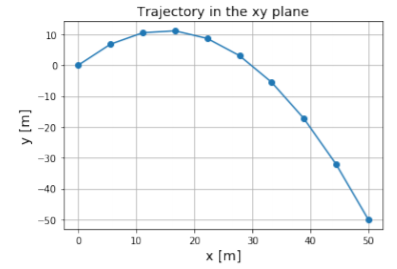
As you can see, the trajectory is a parabola, and corresponds to what you would get when throwing an object with an initial velocity with upwards (positive \(y\)) and horizontal (positive \(x\)) components. If you look at only the \(y\) axis, you will see that the object first goes up, then turns around and goes back down. This is exactly what happens when you throw a ball upwards, independently of whether the object is moving in the \(x\) direction. In the \(x\) direction, the object just moves with a constant velocity. The points on the graph are drawn for constant time intervals (the time between each point, \(\Delta t\) is constant). If you look at the distance between points projected onto the \(x\) axis, you will see that they are all equidistant and that along \(x\), the motion corresponds to that of an object with constant velocity.

Exercise \(\PageIndex{2}\)

In Example 4.1.1, what is the velocity vector exactly at the top of the parabola in Figure \(\PageIndex{2}\)?

1. \(\stackrel{\rightarrow}{v} = (10\text{m/s})\stackrel{ˆ}{x}+(15\text{m/s})\stackrel{ˆ}{y}\)
2. \(\stackrel{\rightarrow}{v} = (15 m/s)\stackrel{ˆ}{y}\)
3. \(\stackrel{\rightarrow}{v} = (10 m/s)\stackrel{ˆ}{x}\)
4. None of the above

Answer

C.

Example \(\PageIndex{2}\)

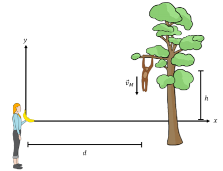
A monkey is hanging from a tree branch and you want to feed the monkey by throwing it a banana (Figure \(\PageIndex{3}\)). You know that the monkey is easily frightened and will let go of the tree branch the instant you throw the banana. The monkey is a horizontal distance \(d\) away and a height \(h\) above the point from which you release the banana when you throw it. At what angle with respect to the horizontal should you throw the banana so that the banana reaches the monkey?

Figure \(\PageIndex{3}\): Feeding a monkey in a tree.

Solution

This question is asking us to find the angle, \(\theta\), between the banana’s initial velocity vector, \(\vec v_{0B}\), and the horizontal for the banana to hit the monkey. This angle is given by the horizontal (\(v_{B0x}\)) and vertical (\(v_{B0y}\)) components of the initial velocity vector of the banana:

\[\begin{aligned} \tan\theta&=\frac{v_{B0y}}{v_{B0x}}\end{aligned}\]

In order for the banana to hit the monkey, and the banana and the monkey must be in the same place at the same time at some time, \(t\). Our approach will be as follows: we will start by finding equations that describe the \(x\) and \(y\) position of the monkey and of the banana. Then, we will use our conditions for a successful “hit” to find the ratio (\(\tan\theta=v_{B0y}/v_{B0x}\)) that we want for our initial throw, and use that to find \(\theta\).

First, we define a coordinate system. We choose the origin to be where the banana is released. We let \(y\) be in the vertical direction (positive upwards) and let \(x\) be in the horizontal direction (positive towards the monkey), as shown in Figure \(\PageIndex{3}\).

We treat the \(x\) and \(y\) components of the banana and monkey’s velocity and position vectors as independent. The monkey’s motion has only a vertical component. The \(y\) component of the monkey’s acceleration is the acceleration due to gravity, \(a_y=-9.8\text{m/s^2}= -g\), which is negative, since gravity produces an acceleration in the negative \(y\) direction. The \(y\) component of the monkey’s initial position is \(y_{M0}=h\) and the \(y\) component of its initial velocity is \(v_{M0y}=0\). The \(y\) component of the monkey’s position as a function of time, \(y_M(t)\), is given by:

\[\begin{aligned} y_M(t)&=y_{M0}+v_{My0}t+\frac{1}{2}a_yt^2\\[4pt] &=h+(0)-\frac{1}{2}gt^2\end{aligned}\]

The horizontal position of the monkey is constant, and is equal to \(x_M(t)=d\).

The banana’s motion has both \(x\) and \(y\) components. There is no acceleration in the \(x\) direction, so the \(x\) component of the banana’s velocity is \(v_{B0x}\) and constant. We defined the banana’s initial \(x\) coordinate to be \(x_{B0}=0\), so the \(x\) position of the banana as a function of time, \(x_B(t)\) is given by:

\[\begin{aligned} x_B(t)&=x_{B0}+v_{B0x}\\[4pt] &=(0)+v_{B0x}t\end{aligned}\]

We defined the initial \(y\) position of the banana to be \(y_{B0}=0\). The \(y\) position of the banana as a function of time, \(y_B(t)\), can thus be described by:

\[\begin{aligned} y_B(t)&=y_{B0}+v_{B0y}t+\frac{1}{2}a_yt^2\\[4pt] &=(0)+v_{B0y}t-\frac{1}{2}gt^2\end{aligned}\]

where \(v_{B0y}\) is the \(y\) component of the banana’s initial velocity and \(a_y=-g\) is the \(y\) component of the banana’s acceleration (due to gravity). Now that we have equations that describe the position of both the banana and the monkey, we can use our conditions for the banana and monkey to be at the same position at the same time. For the monkey and the banana to be in the same position, we need \(y_M(t)=y_B(t)\) and \(x_B(t)=x_M(t) =d\) at some time \(t\).

Setting our equations for \(y_M(t)\) and \(y_B(t)\) equal to one another gives:

\[\begin{aligned} h-\frac{1}{2} gt^2&=v_{0yB}t-\frac{1}{2}gt^2\\[4pt] \therefore h&=v_{0yB}t\end{aligned}\]

And setting \(x_M(t)=d\) equal to \(x_B(t)\) gives:

\[\begin{aligned} \therefore d&=v_{xB}\end{aligned}\]

We can just divide one equation by the other to find:

\[\begin{aligned} \frac{h}{d}&=\frac{v_{0yB}t}{v_{xB}t}\\[4pt] \frac{h}{d}&=\frac{v_{0yB}}{v_{xB}}\end{aligned}\]

This gives us the ratio we are looking for, so we now know that

\[\begin{aligned} \tan\theta&=\frac{h}{d}\\[4pt] \therefore \theta&=\tan^{-1}\left(\frac{h}{d}\right)\end{aligned}\]

This is a somewhat surprising result, as it means that you only need to thrown the banana in the direction of the monkey (that is, aim at the monkey, and throw!). Thus, it will not matter how fast you throw the banana, and you will always hit the monkey if you aimed correctly. When you throw the banana faster, you will hit the monkey higher in its trajectory. If there is no ground for the monkey to hit, you can throw the banana as slowly as you like, and it will eventually catch up with the monkey when the banana reaches \(x=d\).

Relative motion

In the previous chapter, we examined how to convert the description of motion from one reference frame to another. Recall the one dimensional situation where we described the position of an object, \(A\), using an axis \(x\) as \(x^A(t)\). Suppose that the reference frame, \(x\), is moving with a constant speed, \(v'^B\), relative to a second reference frame, \(x'\). We found that the position of the object is described in the \(x'\) reference frame as:

\[\begin{aligned} x'^A(t)=v'^Bt+x^A(t)\end{aligned}\]

if the origins of the two systems coincided at \(t=0\). The equation above simply states that the distance of the object to the \(x'\) origin is the sum of the distance from the \(x'\) origin to the \(x\) origin and the distance from the \(x\) origin to the object.

In two dimensions, we proceed in exactly the same way, but use vectors instead:

\[\begin{aligned} \vec r'^A(t) = \vec v'^Bt+\vec r^A(t)\end{aligned}\]

where \(r^A(t)\) is the position of the object as described in the \(xy\) reference frame, \(\vec v'^B\), is the velocity vector describing the motion of the origin of the \(xy\) coordinate system relative to an \(x'y'\) coordinate system and \(\vec r'^A(t)\) is the position of the object in the \(x'y'\) coordinate system. We have assumed that the origins of the two coordinate systems coincided at \(t=0\) and that the axes of the coordinate systems are parallel (\(x\) parallel to \(x'\) and \(y\) parallel to \(y'\)).

Note that the velocity of the object in the \(x'y'\) system is found by adding the velocity of \(xy\) relative to \(x'y'\) and the velocity of the object in the \(xy\) frame (\(\vec v^A(t)\)):

\[\begin{aligned} \frac{d}{dt}\vec r'^A(t) &=\frac{d}{dt}(\vec v'^Bt+\vec r^A(t))\\[4pt] &=\vec v'^B+\vec v^A(t)\end{aligned}\]

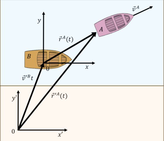
As an example, consider the situation depicted in Figure \(\PageIndex{4}\). Brice is on a boat off the shore of Nice, with a coordinate system \(xy\), and is describing the position of a boat carrying Alice. He describes Alice’s position as \(\vec r^A(t)\) in the \(xy\) coordinate system. Igor is on the shore and also wishes to describe Alice’s position using the work done by Brice. Igor sees Brice’s boat move with a velocity \(\vec v'^B\) as measured in his \(x'y'\) coordinate system. In order to find the vector pointing to Alice’s position \(\vec r'^A(t)\), he adds the vector from his origin to Brice’s origin (\(\vec v'^B t\)) and the vector from Brice’s origin to Alice \(\vec r^A(t)\).

Figure \(\PageIndex{4}\): Example of converting from one reference frame to another in two dimensions using vector addition.

Writing this out by coordinate, we have:

\[\begin{aligned} x'^A(t)&=v'^B_xt+x^A(t)\\[4pt] y'^A(t)&=v'^B_yt+y^A(t)\end{aligned}\]

and for the velocities:

\[\begin{aligned} v_x'^A(t)&=v'^B_x+v_x^A(t)\\[4pt] v_y'^A(t)&=v'^B_y+v_y^A(t)\end{aligned}\]

Exercise \(\PageIndex{3}\)

You are on a boat and crossing a North-flowing river, from the East bank to the West bank. You point your boat in the West direction and cross the river. Chloe is watching your boat cross the river from the shore, in which direction does she measure your velocity vector to be?

1. In the North direction.
2. In the West direction.
3. A combination of North and West directions.

Answer

C.

Footnotes

1. Where a constant vector means that both the magnitude and direction are constant in time.