
4.4: Circular motion
- Page ID
- 19383
We often consider the motion of an object around a circle of fixed radius, \(R\). In principle, this is motion in two dimensions, as a circle is necessarily in a two dimensional plane. However, since the object is constrained to move along the circumference of the circle, it can be thought of (and treated as) motion along a one dimensional axis that is curved.
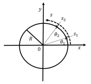
Figure \(\PageIndex{1}\) shows how we can describe motion along a circle of radius, \(R\). We could use \(x(t)\) and \(y(t)\) to describe the position on the circle, however, \(x(t)\) and \(y(t)\) are no longer independent since they have to correspond to the coordinates of points on a circle:
\[\begin{aligned} x^2(t)+y^2(t)=R^2\end{aligned}\]
Instead of using \(x\) and \(y\), we could think of an axis that is bent around the circle (as shown by the curved arrow in Figure \(\PageIndex{1}\), the \(s\) axis). The \(s\) axis is such that \(s=0\) where the circle intersects the \(x\) axis, and the value of \(s\) increases as we move counter-clockwise along the circle. Distance along the \(s\) axis thus corresponds to the distance along the circumference of the circle.
Another variable that could be used for position instead of \(s\) is the angle, \(\theta\), between the position vector of the object and the \(x\) axis, as illustrated in Figure \(\PageIndex{1}\). If we express the angle \(\theta\) in radians, then it is easy to convert between \(s\) and \(\theta\). Recall, an angle in radians is defined as the length of an arc subtended by that angle divided by the radius of the circle. We thus have:
\[\theta(t)=\frac{s(t)}{R}\]
In particular, if the object has gone around the whole circle, then \(s=2\pi R\) (the circumference of a circle), and the corresponding angle is, \(\theta=\frac{2\pi R}{R}=2\pi\), namely 360.
By using the angle, \(\theta\), instead of \(x\) and \(y\), we are effectively using polar coordinates, with a fixed radius. As we already saw, the \(x\) and \(y\) positions are related to \(\theta\) by:
\[\begin{aligned} x(t) &= R\cos(\theta(t))\\[4pt] y(t) &= R\sin(\theta(t))\\[4pt]\end{aligned}\]
where \(R\) is a constant. For an object moving along the circle, we can write its position vector, \(\vec r(t)\), as:
\[\begin{aligned} \vec r(t)&= \begin{pmatrix} x(t) \\[4pt] y(t) \\[4pt] \end{pmatrix} =R \begin{pmatrix} \cos(\theta(t)) \\[4pt] \sin(\theta(t)) \\[4pt] \end{pmatrix}\end{aligned}\]
and the velocity vector is thus given by:
\[\begin{aligned} \vec v(t) &=\frac{d}{dt}\vec r(t) =\frac{d}{dt} R \begin{pmatrix} \cos(\theta(t)) \\[4pt] \sin(\theta(t)) \\[4pt] \end{pmatrix} \\[4pt] &= R \begin{pmatrix} \frac{d}{dt}\cos(\theta(t)) \\[4pt] \frac{d}{dt}\sin(\theta(t)) \\[4pt] \end{pmatrix} \\[4pt] &= R \begin{pmatrix} -\sin(\theta(t))\frac{d\theta}{dt} \\[4pt] \cos(\theta(t))\frac{d\theta}{dt} \\[4pt] \end{pmatrix} \\[4pt] \end{aligned}\]
where we used the Chain Rule to calculate the time derivatives of the trigonometric functions (since \(\theta(t)\) is function of time). We can write this in component form:
\[v_x = -R\sin(\theta(t))\frac{d\theta}{dt}\]
\[ v_y = R\cos(\theta(t))\frac{d\theta}{dt}\]
The magnitude of the velocity vector is given by:
\[\begin{aligned} ||\vec v|| &=\sqrt{ v_x^2+v_y^2}\\[4pt] &=\sqrt{ \left(-R\sin(\theta(t))\frac{d\theta}{dt}\right)^2+\left(R\cos(\theta(t))\frac{d\theta}{dt}\right)^2}\\[4pt] &=\sqrt{ R^2\left( \frac{d\theta}{dt}\right)^2[\sin^2(\theta(t))+\cos^2(\theta(t)]}\\[4pt] &=R\left |\frac{d\theta}{dt}\right|\end{aligned}\]
The position and velocity vectors are illustrated in Figure \(\PageIndex{2}\) for an angle \(\theta\) in the first quadrant (\(0<\theta<\frac{\pi}{2}\)).
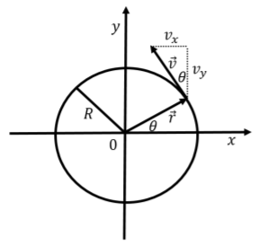
In this case, you can note that the \(x\) component of the velocity is negative (from the diagram and from Equation 4.4.2). From Equations 4.4.2 and 4.4.3, you can also see that \(\frac{|v_x|}{|v_y|}=\tan(\theta)\), which is illustrated in Figure \(\PageIndex{2}\), showing that the velocity vector is tangent to the circle and perpendicular to the position vector. This is always the case for motion along a circle.
We can simplify our description of motion along the circle by using either \(s(t)\) or \(\theta(t)\) instead of the vectors for position and velocity. If we use \(s(t)\) to represent position along the circumference (\(s=0\) where the circle intersects the \(x\) axis), then the velocity along the \(s\) axis is:
\[\begin{aligned} v_s(t)&=\frac{d}{dt}s(t)\\[4pt] &=\frac{d}{dt}R\theta(t)\\[4pt] &=R\frac{d\theta}{dt}\end{aligned}\]
where we used the fact that \(\theta=s/R\) to convert from \(s\) to \(\theta\). The velocity along the \(s\) axis is thus precisely equal to the magnitude of the two-dimensional velocity vector (derived above), which makes sense since the velocity vector is tangent to the circle (and thus in the \(s\) “direction”).
If the object has a constant speed, \(v_s\), along the circle and started at a position along the circumference \(s=s_0\), then its position along the \(s\) axis can be described using 1D kinematics:
\[\begin{aligned} s(t)=s_0+v_st\end{aligned}\]
or, in terms of \(\theta\):
\[\begin{aligned} \theta(t)&=\frac{s(t)}{R}=\frac{s_0}{R}+\frac{v_s}{R}t\\[4pt] &=\theta_0 + \frac{d\theta}{dt}t\\[4pt] &=\theta_0 + \omega t \\[4pt] \therefore\omega &= \frac{d\theta}{dt}\end{aligned}\]
where we introduced \(\theta_0\) as the angle corresponding to the position \(s_0\), and we introduced \(\omega=\frac{d\theta}{dt}\), which is analogous to velocity, but for an angle. \(\omega\) is called the angular velocity and is a measure of the rate of change of the angle \(\theta\) (as it is the time derivative of the angle). The relation between the “linear” velocity \(v_s\) (the magnitude of the velocity vector, which corresponds to the velocity in the direction tangent to the circle) and \(\omega\) is:
\[\begin{aligned}v_s=R\frac{d\theta}{dt}=R\omega \end{aligned}\]
Similarly, if the object is accelerating, we can define an angular acceleration, \(\alpha(t)\), as the rate of change of the angular velocity:
\[\begin{aligned} \alpha(t)=\frac{d\omega}{dt}\end{aligned}\]
which can directly be related to the acceleration in the \(s\) direction, \(a_s(t)\):
\[\begin{aligned} a_s(t) &= \frac{d}{dt}v_s\\[4pt] &=\frac{d}{dt}\omega R=R\frac{d\omega}{dt}\\[4pt] a_s(t)&=R\alpha \end{aligned}\]
Thus, the linear quantities (those along the \(s\) axis) can be related to the angular quantities by multiplying the angular quantities by \(R\):
\[s=R\theta\]
\[v_{s}=R\omega\]
\[a_{s}=R\alpha\]
If the object started at \(t=0\) with a position \(s=s_0\) (\(\theta=\theta_0\)), and an initial linear velocity \(v_{0s}\) (angular velocity \(\omega_0\)), and has a constant linear acceleration around the circle, \(a_s\) (angular acceleration, \(\alpha\)), then the position of the object can be described using either the linear or the angular quantities:
\[\begin{aligned} s(t) &= s_0+v_{s0}t+\frac{1}{2}a_s t^2\\[4pt] \theta(t) &= \theta_0+\omega_0t+\frac{1}{2}\alpha t^2\end{aligned}\]
As you recall from Section 4.3, we can compute the acceleration vector and identify components that are parallel and perpendicular to the velocity vector:
\[\begin{aligned} \vec a&=\vec a_{\parallel}(t) + \vec a_{\bot}(t)\\[4pt] &=\frac{dv}{dt}\hat v(t)+v\frac{d\hat v}{dt}\\[4pt]\end{aligned}\]
The first term, \(\vec a_{\parallel}(t)=\frac{dv}{dt}\hat v(t)\), is parallel to the velocity vector \(\hat v\), and has a magnitude given by:
\[\begin{aligned} ||\vec a_{\parallel}(t)||&=\frac{dv}{dt}=\frac{d}{dt} v(t)=\frac{d}{dt} R\omega=R\alpha\end{aligned}\]
That is, the component of the acceleration vector that is parallel to the velocity is precisely the acceleration in the \(s\) direction (the linear acceleration). This component of the acceleration is responsible for increasing (or decreasing) the speed of the object and is zero if the object goes around the circle with a constant speed (linear or angular).
As we saw earlier, the perpendicular component of the acceleration, \(\vec a_{\bot}(t)\), is responsible for changing the direction of the velocity vector (as the object continuously changes direction when going in a circle). When the motion is around a circle, this component of the acceleration vector is called “centripetal” acceleration (i.e. acceleration pointing towards the center of the circle, as we will see). We can calculate the centripetal acceleration in terms of our angular variables, noting that the unit vector in the direction of the velocity is \(\hat v=-\sin(\theta)\hat x+\cos(\theta)\hat y\):
\[\begin{aligned} \vec a_{\bot}(t)&=v\frac{d\hat v}{dt}\nonumber\\[4pt] &=(\omega R)\frac{d}{dt} \left[-\sin(\theta)\hat x+\cos(\theta)\hat y\right]\nonumber\\[4pt] &=\omega R \left[-\frac{d}{dt}\sin(\theta)\hat x+\frac{d}{dt}\cos(\theta)\hat y\right]\nonumber\\[4pt] &=\omega R \left[-\cos(\theta)\frac{d\theta}{dt}\hat x-\sin(\theta)\frac{d\theta}{dt}\hat y\right]\nonumber\\[4pt] &=\omega R [-\cos(\theta)\omega\hat x-\sin(\theta)\omega\hat y]\nonumber\end{aligned}\]
\[\stackrel{\rightarrow}{a} _{\bot}(t)=ω^{2}R[-\cos(\theta)\hat x-\sin(\theta)\hat y\]
where you can easily verify that the vector \([-\cos(\theta)\hat x-\sin(\theta)\hat y]\) has unit length and points towards the center of the circle (when the tail is placed on a point on the circle at angle \(\theta\)). The centripetal acceleration thus points towards the center of the circle and has magnitude:
\[a_c(t) = ||\vec a_{\bot}(t)||=\omega^2(t) R = \frac{v^2(t)}{R}\]
where in the last equal sign, we wrote the centripetal acceleration in terms of the speed around the circle (\(v=||\vec v||=v_s\)).
If an object goes around a circle, it will always have a centripetal acceleration (since its velocity vector must change direction). In addition, if the object’s speed is changing, it will also have a linear acceleration, which points in the same direction as the velocity vector (it changes the velocity vector’s length but not its direction).
A vicuña is going clockwise around a circle that is centerd at the origin of an \(xy\) coordinate system that is in the plane of the circle. The vicuña runs faster and faster around the circle. In which direction does its acceleration vector point just as the vicuña is at the point where the circle intersects the positive \(y\) axis?
- In the negative \(y\) direction.
- In the positive \(y\) direction.
- A combination of the positive \(y\) and positive \(x\) directions.
- A combination of the negative \(y\) and positive \(x\) directions.
- A combination of the negative \(y\) and negative \(x\) directions.
- Answer
- D.
Period and Frequency
When an object is moving around in a circle, it will typically complete more than one revolution. If the object is going around the circle with a constant speed, we call the motion “uniform circular motion”, and we can define the period and frequency of the motion.
The period, \(T\), is defined to be the time that it takes to complete one revolution around the circle. If the object has constant angular speed \(\omega\), we can find the time, \(T\), that it takes to complete one full revolution, from \(\theta=0\) to \(\theta=2\pi\):
\[\begin{aligned} \omega&=\frac{\Delta \theta}{T}=\frac{2\pi}{T}\nonumber\end{aligned}\]
\[T=\frac{2\pi}{\omega}\]
We would obtain the same result using the linear quantities; in one revolution, the object covers a distance of \(2\pi R\) at a speed of \(v\):
\[\begin{aligned} v&=\frac{2\pi R}{T}\\[4pt] T&=\frac{2\pi R}{v}=\frac{2\pi R}{\omega R}=\frac{2\pi}{\omega}\end{aligned}\]
The frequency, \(f\), is defined to be the inverse of the period:
\[\begin{aligned} f&=\frac{1}{T}=\frac{\omega}{2\pi}\end{aligned}\]
and has SI units of \(\text{Hz}=\text{s}^{-1}\). Think of frequency as the number of revolutions completed per second. Thus, if the frequency is \(f=1\text{Hz}\), the object goes around the circle once per second. Given the frequency, we can of course obtain the angular velocity:
\[\begin{aligned} \omega = 2\pi f\end{aligned}\]
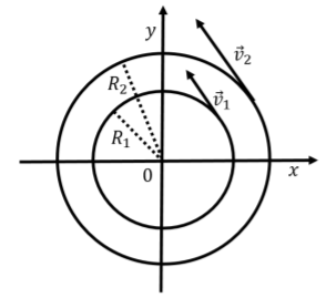
which is sometimes called the “angular frequency” instead of the angular velocity. The angular velocity can really be thought of as a frequency, as it represents the “amount of angle” per second that an object covers when going around a circle. The angular velocity does not tell us anything about the actual speed of the object, which depends on the radius \(v=\omega R\). This is illustrated in Figure \(\PageIndex{3}\), where two objects can be traveling around two circles of radius \(R_1\) and \(R_2\) with the same angular velocity \(\omega\). If they have the same angular velocity, then it will take them the same amount of time to complete a revolution. However, the outer object has to cover a much larger distance (the circumference is larger), and thus has to move with a larger linear speed.
A motor is rotating at \(3000\text{ rpm}\), what is the corresponding frequency in Hz?
- \(5\text{ Hz}\)
- \(50\text{ Hz}\)
- \(500\text{ Hz}\)
- Answer
- B.
There's a trick I like to use to remember how linear and angular velocities work. Figure 4.4.4 shows your hand in two positions, which we call (1) and (2).
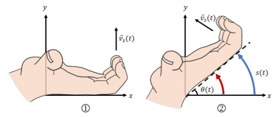
Let’s say you want to describe the location of your fingers in (2). Start by putting your hand in position (1). This is the position where \(\theta=0\) and \(s=0\). Imagine that your wrist (or your thumb, whichever you prefer) is fixed at the origin. If you keep your fingers perpendicular to your hand, they will always point in the positive \(s\) direction.
Imagine that you have a blue glob of paint on the back of your pinky. Rotate your hand until it is in position (2). The length of the curve that the paint makes is the value of \(s\). The angle between the back of your hand and the positive \(x\)-axis is \(\theta\). Now, imagine that there is a red glob of paint at your palm. It takes the same amount of time for your palm to get from position (1) to position (2) as it does for your fingers. Since they both go through the same angle \(\theta\) in the same amount of time, the angular velocity, \(\omega\) must be the same for both. However, the blue line left by your fingers will be much longer than the red line left by your palm. Your fingers traveled a greater distance than your palm in the same amount of time, so they must have a greater linear velocity, \(v_s\). The further you are from your thumb, the greater the linear velocity will be, which we know from the formula \(v_s=R\omega\).
If you kept rotating your hand around the circle, you would see that your fingers always point in the same direction as your linear velocity. This means that if you are using Cartesian coordinates, the direction of your linear velocity is always changing.
There are a couple of limitations to this trick. Remember that this only works for circular motion (the radius \(R\) must be constant) and that if you are moving in the negative \(s\) direction, your fingers will point antiparallel to the linear velocity.