14.2: Mathematical Description of a Wave

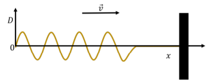
In order to describe the motion of a wave through a medium, we can describe the motion of the individual particles of the medium as the wave passes through. Specifically, we describe the position of each particle using its displacement, \(D\), from its equilibrium position. Consider our rope example in which a sine wave is propagating through a medium (the rope) in the positive \(x\) direction, as shown in Figure \(\PageIndex{1}\).

Figure \(\PageIndex{1}\): The displacement (\(D\)) of points at different positions (\(x\)) on a rope as a sine wave passes through.

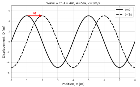
The displacement, \(D\), of each point at position, \(x\), in the medium is shown on the vertical axis of Figure \(\PageIndex{2}\). The solid black line corresponds to a snapshot of the wave at time \(t=0\). The wave has an amplitude, \(A=5\text{m}\), a velocity, \(v=1\text{m/s}\), and a wavelength, \(\lambda=4\text{m}\). The dotted line corresponds to a snapshot of the wave one second later, at \(t=1\text{s}\), when the wave has moved to the right by a distance \(vt=1\text{m}\).

Figure \(\PageIndex{2}\): Displacement as a function of position for particles in a medium as a wave passes through. The dotted line shows the displacement as a function of time \(1\text{ s}\) after the solid line, and corresponds to a wave traveling towards the right.

It is important to note that Figure \(\PageIndex{2}\) is not restricted to describing transverse waves, even if the illustration suggests that the particles’ displacements (vertical axis) are perpendicular to the direction of propagation of the wave (horizontal). The quantity, \(D\), that is plotted on the vertical axis corresponds to the displacement of a particle from its equilibrium position. That displacement could correspond to the longitudinal displacement of a particle in a longitudinal wave.

At time \(t=0\) (solid line), the displacement of each point in the medium, \(D(x, t=0)\), as a function of their distance from the origin, \(x\), can be described by a sine function:

\[D(x,t=0)=A\sin\left(\frac{2\pi}{\lambda}x \right) \]

This corresponds to the displacement being 0 at the origin and at any position, \(x\), that is a multiple of the wavelength, \(\lambda\).

If the wave moves with velocity \(v\) in the positive \(x\) direction, then at time \(t\), the sine function in Figure \(\PageIndex{2}\) will have shifted to the right by an amount \(vt\) (dotted line). The displacement of a point located at position \(x\) at time \(t\) will be the same as the displacement of the point at position \(x-vt\) at time \(t=0\). For example, in Figure \(\PageIndex{2}\) the displacement of the point \(x=2\text{m}\) at time \(t=1\text{s}\) is the same as the displacement of the point at position \(x-vt=1\text{m}\) at \(t=0\).

We can state this condition as:

\[\begin{aligned} D(x,t) = D(x-vt, t=0)\end{aligned}\]

That is, at some time \(t\), the displacement of a point at position \(x\) is found by finding the position of the point at \(x-vt\) at \(t=0\). We already have an equation to find the displacement of a point at \(t=0\). Using the above condition, we can modify Equation 14.2.1 to write a function for the displacement of a point at position \(x\) at time \(t\):

\[\begin{aligned} D(x,t) = A\sin\left( \frac{2\pi}{\lambda}(x-vt) \right)\end{aligned}\]

Noting that \(v/\lambda= 1/T\), we can write this as:

\[\begin{aligned} D(x,t) = A\sin\left( \frac{2\pi x}{\lambda}- \frac{2\pi t}{T} \right)\end{aligned}\]

In the above derivation, we assumed that at time \(t=0\), the displacement at \(x=0\) was \(D(x=0, t=0)=0\). In general, the displacement could have any value at \(x=0\) and \(t=0\), so we can allow the wave to shift left or right by including a phase, \(\phi\), which can be determined from the displacement at \(x=0\) and \(t=0\):

\[ D(x,t) = A\sin\left(\frac{2\pi x}{\lambda}-\frac{2\pi t}{T}+\phi \right)\]

where \(\phi=0\) corresponds to the displacement being zero at \(x=0\) and \(t=0\).

Exercise \(\PageIndex{1}\)

What is the value of the phase \(\phi\) if the displacement of the point at \(x=0\) is \(D=A/2\) at time \(t=0\)?

1. \(\pi/6\).
2. \(\pi/4\).
3. \(\pi/3\).
4. \(\pi/2\).

Answer

The equation above is written in terms of the wavelength, \(\lambda\), and period, \(T\), of the wave. Often, one uses the “wave number”, \(k\), and the “angular frequency”, \(\omega\), to describe the wave. These are defined as:

\[k=\frac{2\pi}{\lambda}\]

\[\omega = \frac{2\pi}{T}\]

Using the wave number and the angular frequency removes the factors of \(2\pi\) in the expression for \(D(x,t)\), which can now be written as:

\[D(x,t)=A\sin (kx-\omega t+\phi )\]

It is important to note that the wave number, \(k\), has no relation to the spring constant that we used for springs.

Using Equation 14.1.1, we can also relate the wave number and angular frequency to the speed of the wave:

\[\begin{aligned} v = \frac{\lambda}{T}=\frac{\frac{2\pi}{k}}{\frac{2\pi}{\omega}}=\frac{\omega}{k}\end{aligned}\]

The Wave Equation

In Chapter 13, we saw that any physical system whose position, \(x\), satisfies the following equation:

\[\begin{aligned} \frac{d^2x}{dt^2}=-\omega^2 x\end{aligned}\]

will undergo simple harmonic motion with angular frequency \(\omega\), and that \(x(t)\) can be modeled as:

\[\begin{aligned} x(t) = A\cos(\omega t + \phi)\end{aligned}\]

Similarly, any system, where the displacement of a particle as a function of position and time, \(D(x,t)\), satisfies the following equation:

\[\frac{\partial ^{2}D}{\partial x^{2}}=\frac{1}{v^{2}}\frac{\partial ^{2}D}{\partial t^{2}}\]

is described by a wave that propagates with a speed \(v\). The equation above is called the “one-dimensional wave equation” and would be obtained from modeling the dynamics of the system, just as the equation of motion for a simple harmonic oscillator can be obtained from Newton’s Second Law. For the harmonic oscillator, the properties of the system (e.g. mass and spring constant) determine the angular frequency, \(\omega\). For a wave, the properties of the medium determine the speed of the wave, \(v\).

We use partial derivatives in the wave equation instead of total derivatives because \(D(x,t)\) is multivariate. A possible solution to the one-dimensional wave equation is:

\[\begin{aligned} D(x,t) = A\sin\left( kx -\omega t + \phi \right)\end{aligned}\]

which is the function that we used in the previous section to describe a sine wave.

Furthermore, if multiple solutions to the wave equation, \(D_1(x,t)\), \(D_2(x,t)\), etc, exist, then any linear combination, \(D(x,t)\), of the solutions will also be a solution to the wave equation:

\[\begin{aligned} D(x,t) = a_1D_1(x,t)+a_2D_2(x,t)+a_3D_3(x,t)+\dots\end{aligned}\]

This last property is called “the superposition principle”, and is the result of the wave equation being linear in \(D\) (it does not depend on \(D^2\), for example). It is easy to check, for example, that if \(D_1(x,t)\) and \(D_2(x,t)\) satisfy the wave equation, so does their sum.

In three dimensions, the displacement of a particle in the medium depends on its three spatial coordinates, \(D(x,y,z,t)\), and the wave equation in Cartesian coordinates is given by:

\[\begin{aligned} \frac{\partial ^{2}D}{\partial x^{2}}+\frac{\partial ^{2}D}{\partial y^{2}}+\frac{\partial ^{2}D}{\partial z^{2}}&=\frac{1}{v^2}\frac{\partial ^{2}D}{\partial t^{2}}\\[4pt]\end{aligned}\]

There are many functions that can satisfy this equation, and the best choice will depend on the physical system being modeled and the properties of the wave that one wishes to describe.