
15.3: Hydrodynamics
- Page ID
- 19474
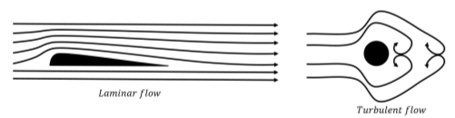
In the previous sections we developed “hydrostatic” models for fluids when those fluids are at rest (in some inertial reference frame). In this section, we develop “hydrodynamic” models to discuss what happens when fluids flow. We will restrict our models to fluids that flow in a “laminar” fashion, rather than a “turbulent” fashion.
Laminar flow is the flow of a fluid when each particle in the fluid follows a path that can be represented by a line (a “streamline”). Turbulent flow is the flow of a fluid where particles can follow rather complex paths, usually involving “Eddy currents” (little whirlpools). The two types of flow are illustrated in Figure \(\PageIndex{1}\).
Continuity of flow
Consider the laminar flow of a fluid through a pipe whose cross-sectional area narrows from \(A_{1}\) to \(A_{2}\) in the direction of flow, as illustrated in Figure \(\PageIndex{2}\).
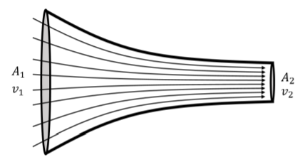
The particles that make up the fluid have a speed \(v_{1}\) at the wide end of the pipe and speed \(v_{2}\) at the narrow end. The equation of continuity is based on the premise that the fluid that enters the pipe must exit the pipe, as there is nowhere else for the fluid to go. That is, if during a period of time, \(∆t\), a mass, \(∆m\), of fluid enters the wide end of the pipe, then during that same period of time, the same mass of fluid must exit the narrow end of the pipe.
During a period of time, \(∆t\), the fluid at the wide end of the pipe will travel a distance \(l_{1} = v_{1}∆t\). Thus, a volume of fluid, \(∆V_{1}\), will enter the wide end of the pipe:
\[\begin{aligned} \Delta V_{1}=A_{1}l_{1}=A_{1}v_{1}\Delta t \end{aligned}\]
Similarly, during that period of time, a volume \(∆V_{2}\) will exit the narrow end of the pipe:
\[\begin{aligned} \Delta V_{2}=A_{2}l_{2}=A_{2}v_{2}\Delta t \end{aligned}\]
If the fluid is compressible, its density can change. Let \(ρ_{1}\) be the density of the fluid at the wide end of the pipe and \(ρ_{2}\) be the density of the fluid at the narrow end. The mass of fluid, \(∆m\), entering the wide end of the pipe is given by:
\[\begin{aligned} \Delta m = \rho _{1}\Delta V_{1}=\rho _{1}A_{1}v_{1}\Delta t \end{aligned}\]
The mass of fluid exiting the narrow end of the pipe is given by:
\[\begin{aligned} \Delta m = \rho _{2}\Delta V_{2} = \rho _{2}A_{2}v_{2}\Delta t\end{aligned}\]
The mass of fluid entering the wide end of the pipe must equal the mass exiting the narrow end of the pipe:
\[\begin{aligned} \rho _{1}A_{1}v_{1}\Delta t = \rho _{2}A_{2}v_{2}\Delta t \end{aligned}\]
Leading to the equation of continuity:
\[\rho _{1}A_{1}v_{1}=\rho _{2}A_{2}v_{2}\]
The quantity \(ρAv\) has dimensions of mass per time, and corresponds to the mass of fluid passing through a cross section \(A\) per unit time.
If the fluid is incompressible, as are most liquids, then the density is the same on both sides of the pipe, and the equation simplifies to:
\[A_{1}v_{1}=A_{2}v_{2}\qquad\text{(Incompressible fluid)}\]
For a liquid, we can define the “volumetric flow”, \(Q\), as:
\[\begin{aligned} Q=Av \end{aligned}\]
where \(A\) is the cross-sectional area of the surface through which a fluid with speed, \(v\), flows1. \(Q\) has the dimension of volume per time, and corresponds to the volume of fluid passing through the cross section \(A\) per unit time. For an incompressible fluid, the equation of continuity is thus equivalent to stating that the volumetric flow, \(Q\), of the fluid is a constant.
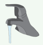
When water flows out of your faucet, you observe that the stream of water gets narrower as the water moves down, as shown in Figure \(\PageIndex{3}\). Why is this?
- The atmospheric pressure increases as the waters moves downwards, so the stream of water is more and more compressed.
- As the water accelerates due to gravity, the cross-sectional area of the flowing water must reduce in order to preserve a constant flow rate.
- Answer
Your garden hose has a diameter of \(D = 2\text{ cm}\). How fast must water flow out of the hose if you are to fill a \(5\text{ l}\) bucket in one minute?
Solution
We need the volume flow rate from the hose to be \(Q = 5\text{ l/min}\). We can convert this to SI units:
\[\begin{aligned} Q=(5\text{l/min})\left( \frac{1}{1000}\text{m}^{3}\text{/l} \right)\left( \frac{1}{60}\text{min/s} \right)=\frac{5}{6\times 10^{4}}\text{m}^{3}\text{/s} = 8.3\times 10^{-5}\text{m}^{3}\text{/s} \end{aligned}\]
Since we know the area of the hose, we can determine the speed of the water to achieve the given flow rate:
\[\begin{aligned} Q&=Av=\pi \left(\frac{D}{2} \right)^{2}v \\[4pt] \therefore v&=\frac{Q}{\pi \left( \frac{D}{2} \right)^{2}}=\frac{(8.3\times 10^{-5}\text{m}^{3}\text{/s})}{\pi (0.01\text{m})^{2}}=0.265\text{m/s} \end{aligned}\]
Bernoulli's Principle
In this section, we examine how the pressure and speed of a fluid change as a the fluid flows. We will restrict ourselves to discussing the laminar flow of an incompressible fluid with no friction. Bernoulli was the first to quantitatively describe the flow of incompressible fluids, and we will show in this section how to derive “Bernoulli’s Principle”.
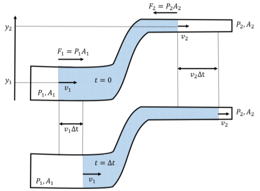
Consider the laminar flow of an incompressible fluid through a pipe that changes height, from \(y_{1}\) to \(y_{2}\), as well as cross-sectional area, from \(A_{1}\) to \(A_{2}\), as shown in Figure \(\PageIndex{4}\). The figure shows an element of fluid, in blue, as it moves through the pipe. The top panel corresponds to the location of the fluid element at time \(t = 0\), whereas the bottom panel shows the location of the element of fluid at time \(t = ∆t\).
To model how the fluid moves through this pipe, we can use energy and the Work-Energy Theorem. We start by considering the amount of work done on the element of fluid as it moves from the position in the top panel to the position in the bottom panel.
The fluid that is to the left of the element of fluid exerts a pressure, \(P_{1}\), on the fluid element that leads to a net force, \(\vec F_{1}\), towards the right. Similarly, the fluid to the right of the element of fluid exerts a net force \(\vec F_{2}\) in the opposite direction, due to the pressure \(P_{2}\) on that side of the fluid element.
In a period of time, \(∆t\), the left part of the fluid element will move a distance \(l_{1} = v_{1}∆t\), while the right part of the fluid element will move a distance \(l_{2} = v_{2}∆t\). We can calculate the work done by each force, defining positive work to be in the direction of motion:
\[\begin{aligned} W_{1}&=F_{1}l_{1}=(P_{1}A_{1})(v_{1}\Delta t) \\[4pt] W_{2} &=-F_{2}l_{2}=-(P_{2}A_{2})(v_{2}\Delta t) \end{aligned}\]
Gravity will also do (negative) work on the fluid as it changes height. In a period of time, \(∆t\), a mass of fluid, \(∆m\), will move from position \(y = y_{1}\) to position \(y = y_{2}\). The mass of fluid that changes height is given by the part of the fluid that moves a distance, \(l_{1}\), on the right side of the pipe:
\[\begin{aligned} \Delta m = V_{1}\rho = A_{1}l_{1}\rho = A_{1}v_{1}\Delta t\rho \end{aligned}\]
Because of the equation of continuity, this is also equal to the mass of fluid that moves a distance, \(l_{2}\), on the left side of the pipe:
\[\begin{aligned} \Delta m = V_{2}\rho = A_{2}l_{2}\rho = A_{2}v_{2}\Delta t\rho \end{aligned}\]
since \(A_{1}v_{1}=A_{2}v_{2}\).
The force of gravity will thus do negative work on that mass element:
\[\begin{aligned} W_{g}=-\Delta mg(y_{2}-y_{1})=-(A_{1}v_{1}\Delta t\rho)g(y_{2}-y_{1}) \end{aligned}\]
The net work done on the element of fluid over the time \(∆t\) is thus:
\[\begin{aligned} W^{net}=W_{1}+W_{2}+W_{g}=P_{1}A_{1}v_{1}\Delta t-P_{2}A_{2}v_{2}\Delta t - A_{1}v_{1}\Delta t \rho g(y_{2}-y_{1}) \end{aligned}\]
Note that, because of the equation of continuity, \(A_{1}v_{1} = A_{2}v_{2}\), we can factor out a \(A_{1}v_{1}\) from each term:
\[\begin{aligned} W^{net}=A_{1}v_{1}\Delta t(P_{1}-P_{2}-\rho g(y_{2}-y_{1})) \end{aligned}\]
The net work done on the fluid must equal the change in kinetic energy, \(∆K\), of the mass element, \(∆m\), from one end of the pipe to the other:
\[\begin{aligned} \begin{aligned} \Delta K&=\frac{1}{2}\Delta mv_{2}^{2} - \frac{1}{2}\Delta mv_{1}^{2} \\[4pt] &=\frac{1}{2}(A_{1}v_{1}\Delta t\rho )(v_{2}^{2}-v_{1}^{2}) \end{aligned} \end{aligned}\]
Using the Work-Energy Theorem, we have:
\[\begin{aligned} W^{net}&=\Delta K \\[4pt] A_{1}v_{1}\Delta t\left(P_{1} - P_{2}-\rho g(y_{2}-y_{1})\right)&=\frac{1}{2}(A_{1}v_{1}\Delta t\rho )(v_{2}^{2}-v_{1}^{2}) \\[4pt] P_{1}-P_{2}-\rho g(y_{2}-y_{1})&=\frac{1}{2}\rho v_{2}^{2}-\frac{1}{2}\rho v_{1}^{2} \end{aligned}\]
We can re-arrange this so that all the quantities for each side of the pipe are on the same side of the equation:
\[\begin{aligned} P_{1}+\frac{1}{2}\rho v_{1}^{2} +\rho gy_{1}=P_{2}+\frac{1}{2}\rho v_{2}^{2}+\rho gy_{2} \end{aligned}\]
Since the locations 1 and 2 that we chose are arbitrary, we can state that, for laminar incompressible flow, the following quantity evaluated at any position is a constant:
\[P+\frac{1}{2}\rho v^{2}+\rho gy = \text{constant}\]
This statement is what we call Bernoulli’s Equation, and is equivalent to conservation of energy for the fluid. If the fluid is not flowing \((v_{1} = v_{2} = 0)\), then this is equivalent to the statement of hydrostatic equilibrium that we derived in Equation 15.1.1:
\[\begin{aligned} P_{1}+\rho gy_{1}&=P_{2}+\rho gy_{2} \\[4pt] \therefore P_{2}-P_{1}=-\rho g(y_{2}-y_{1}) \end{aligned}\]
If the flow of the fluid is at constant height \((y_{2} = y_{1})\), then Bernoulli’s equation can be written as:
\[\begin{aligned} P_{1}+\frac{1}{2}\rho v_{1}^{2}=P_{2}+\frac{1}{2}\rho v_{2}^{2} \end{aligned}\]
If a fluid is flowing at constant height such that \(v_{2} > v_{1}\) (as in Figure \(\PageIndex{2}\)), then \(P_{2} < P_{1}\); that is, the pressure in the fluid is lower if the fluid is flowing faster. Note that \(P\) is the pressure inside the fluid and is not related to the force that would be exerted by the fluid if it were to collide with an object. It makes sense that the fluid has a lower pressure where it is moving faster, because the net force exerted on the fluid is related to the difference in pressure on either side of the fluid. The fluid will accelerate in the direction where pressure decreases, thus it will be moving faster when it is in a region of low pressure.
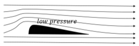
Bernoulli’s principle can be used to describe many phenomena. For example, an airplane wing (technically, an “airfoil”) creates lift because the pressure of the air above the wing is lower than the pressure above the wing. This is illustrated in Figure \(\PageIndex{5}\), which shows that the laminar flow of the air creates a low pressure area above the wing. As the stream lines of air encounter the wing, those that are above the wing get compressed together, which leads to a faster speed of the air above the wing (equation of continuity). The resulting difference in air pressure above and below the wing results in a net upwards force on the wing.
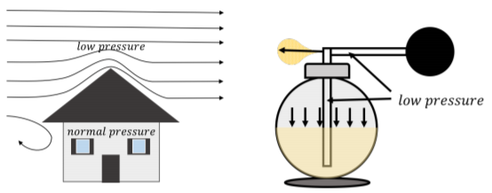
Bernoulli’s principle also describes why the roof can be lifted off of a house in high winds (Figure \(\PageIndex{6}\), left panel). It is not the force of the wind against the roof that blows the roof off of a house; it is the difference in air pressure in the house (normal) and the pressure above the roof (low, due to the flowing wind), that results in a net upwards force on the roof. Bernoulli’s principle is also used to construct atomizers which allow liquid in a bottle to be sprayed (Figure \(\PageIndex{6}\), right panel). For example, perfume bottles often have a bulb connected to a tube/spout. When you squeeze the bulb, it causes the air in the tube to flow quickly, creating a low pressure in the vertical segment of the spout. The liquid is forced up by the pressure in the bottle; once the liquid arrives in the fast flowing air, it is sprayed out along with the air.
When a high speed train is traveling at constant speed, is there a net force on the windows from air pressure?
- No, since the windows are stationary relative to the train, there is no net force on them from air pressure.
- Yes, there is a net outwards force on the windows from air pressure.
- Yes, there is a net inwards force on the windows from air pressure.
- Answer
The following examples illustrate how to apply Bernoulli’s principle.
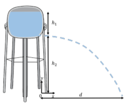
A water tower is constructed so that the bottom of the water tank is a height \(h_{2}\) above the ground, as illustrated in Figure \(\PageIndex{7}\). The water in the tank is at a height \(h_{1}\) from the bottom of the tank. A leak from a hole is found at the base of the tank (the water flows horizontally out of the hole). What is the horizontal distance, \(d\), from the bottom of the tower to where the water from the leak hits the ground? Assume that the water level in the tank is constant and that atmospheric pressure does not change appreciably over the height of the tower.
Solution
The pressure in the water tank leads to the water exiting the bottom of the tank with a horizontal velocity of magnitude, \(v\). That water then undergoes projectile motion on its way to the ground. We can first determine the speed of the water exiting the tank and then use the kinematics for projectile motion to model the distance, \(d\).
We model the flow of the water using a two-dimensional coordinate system with a horizontal \(x\) axis (positive to the right), and a vertical \(y\) axis (positive upwards). We place the origin at the bottom of the water tower, on the ground, below the hole, as shown in Figure \(\PageIndex{7}\).
At the top of tank, at a height \(y = h_{1} + h_{2}\), the water has a speed of zero and is at atmospheric pressure, \(P_{0}\). At the exit of the hole at the bottom of the tank, at a height \(y = h_{2}\), the water has a speed \(v_{2}\) and is also at atmospheric pressure. Using Bernoulli’s equation at the top (1) and bottom (2) of the tank, we have:
\[\begin{aligned} P_{1}+\frac{1}{2}\rho v_{1}^{2}+\rho gy_{1}&=P_{2}+\frac{1}{2}\rho v_{2}^{2}+\rho gy_{2} \\[4pt] P_{0} +(0) +\rho g(h_{1}+h_{2})&=P_{0}+\frac{1}{2}\rho v^{2}+\rho gh_{2} \\[4pt] \therefore v_{2}&=\sqrt{2gh_{1}} \end{aligned}\]
which is exactly the speed that any object falling a distance \(h_{1}\) would have.
Using kinematics, we can find the time that it would take the water to fall a distance \(h_{2}\) (where the water’s velocity is horizontal as it exits the tank):
\[\begin{aligned} h_{2}&=\frac{1}{2}gt^{2} \\[4pt] \therefore t&=\sqrt{\frac{2h_{2}}{g}} \end{aligned}\]
The distance \(d\) covered by the water is thus given by:
\[\begin{aligned} d=v_{2}t=\sqrt{2gh_{1}}\sqrt{\frac{2h_{2}}{g}}=\sqrt{4h_{1}h_{2}} \end{aligned}\]
Discussion
We find that the water coming out of the bottom of the tank, when there is a height, \(h_{1}\), of water above it providing pressure, will have the same speed as that of a particle which has fallen a distance, \(h_{1}\). This is because there is no net pressure difference between the top of the water tank and where the water has exited the hole, so gravity is the only force doing work on the water. Gravity will do work at the same rate on particles of water as on any other particle, so the speed of the water particles at the bottom of the tank is the same as if they had fallen a distance, \(h_{1}\). Again, once the water particles are falling through the air, gravity is the only net force exerted on those particles, so they undergo projectile motion, just as any other particle would.
You measure that water comes out of your kitchen faucet at a rate of \(6\text{ l/min}\). The faucet has a diameter of \(2\text{ cm}\). At what rate will water flow out of your basement faucet, which has a diameter of \(1\text{ cm}\) and is located a height, \(h=\text{ 3 m}\), below your kitchen faucet? Assume that atmospheric pressure, \(P_{0}\), does not change appreciably between your kitchen and basement.
Solution
The water flows out of the kitchen faucet at a speed, \(v_{1}\), where the pressure is atmospheric. If the area of the kitchen faucet is \(A_{1}\) we can determine the speed, \(v_{1}\), from the given flow rate, \(Q_{1} = 6 \text{l/min} = 1 × 10^{−4} \text{m}^{3}\text{/s}\):
\[\begin{aligned} Q_{1}&=A_{1}v_{1} \\[4pt] v_{1}&=\frac{Q_{1}}{A_{1}}=\frac{(1\times 10^{-4}\text{m}^{3}\text{/s})}{\pi (0.01\text{cm})^{2}}=0.318\text{m/s} \end{aligned}\]
The water will flow out of the basement faucet with a speed, \(v_{2}\), where the pressure is also atmospheric, \(P_{0}\). We can use Bernoulli’s equation to relate the flow out of the basement faucet (2) to that at the kitchen faucet (1). We choose the \(y\) axis of a vertical coordinate system such that the basement is located at \(y_{2} = 0\) and the kitchen faucet is located at \(y_{1} = 3\text{ m}\):
\[\begin{aligned} P_{1}+\frac{1}{2}\rho v_{1}^{2}+\rho gy_{1}&=P_{2}+\frac{1}{2}\rho v_{2}^{2}+\rho gy_{2} \\[4pt] P_{0}+\frac{1}{2}\rho v_{1}^{2}+\rho gy_{1}&=P_{0}+\frac{1}{2}\rho v_{2}^{2} \\[4pt] \frac{1}{2}v_{1}^{2}+gy_{1}&=\frac{1}{2}v_{2}^{2} \\[4pt] \therefore v_{2}&=\sqrt{v_{1}^{2}+2gy_{1}} \\[4pt] &=\sqrt{(0.318\text{m/s})^{2}+2(9.8\text{m/s}^{2})(3\text{m})} = 7.67\text{m/s} \end{aligned}\]
The corresponding flow rate at the basement faucet will be:
\[\begin{aligned}Q_{2}=A_{2}v_{2}=\pi(0.005\text{m})^{2}(7.67\text{m/s})=6.03\times 10^{-4}\text{m}^{3}\text{/s}=36.171\text{/min}\end{aligned}\]
Discussion
We find that the flow rate out of the basement faucet is six times that at the kitchen faucet. The speed of the water coming out of the basement faucet is more than \(20\) times the speed of the water at the kitchen faucet. Although it is true that one gets better water pressure out of a faucet that is lower in the building, this change in flow is unrealistically high, and this is a poor model for flow of water in the pipes of your house.
You can easily verify that the speed of the water in different levels of your house does not vary by a factor near \(20\) for a \(3\text{ m}\) change in height (you could compare the flow rate for two faucets with the same diameter). This is because our model neglects the effect of friction as water flows in the pipes; in reality, there is much greater pressure in the pipes than that due to gravity, as well as a gradient in the pressure in your pipes, that will lead to the flow rates being similar in your kitchen and basement.
Viscosity
So far, we have assumed that fluids flow with no friction. In reality, the particles moving in a fluid exert internal friction on each other called “viscosity”. This can be modeled as the friction between different layers of fluid in a laminar flow. For example, you may notice that the water that flows in a wide river flows much faster in the middle of the river than near the river banks, where the water is almost stationary, as shown in Figure \(\PageIndex{8}\).
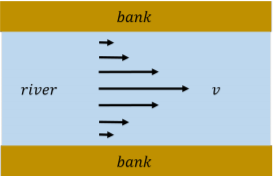
One can model the banks of the river as exerting a frictional force on the layer of water that is in contact with the banks. That layer then exerts a frictional force on the next layer closer to the center of the river, and so on.
One can define a viscosity coefficient, \(η\), based on measuring the force required to pull a plate past another plate when there is a fluid between the plates. Consider two plates that have an area, \(A\), that are a distance \(l\) apart, and contain the fluid of interest between them, as illustrated in Figure \(\PageIndex{9}\).
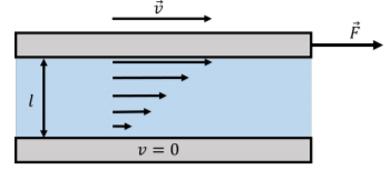
The viscosity of the fluid is defined based on the force that is required to pull the top plate while the bottom plate remains immobile. The layer of fluid directly below the moving plate will move with the plate at a speed, \(v\), while the layer of fluid immediately in contact will the stationary plate will also be stationary. Moving one plate will thus lead to a gradient (a change) in the speed of the fluid as a function of the position between the two plates. The magnitude of the force, \(\vec F\), required to move one plate with speed, \(v\), was empirically determined to be proportional to the area of the plates, \(A\), and the speed, \(v\), while being inversely proportional to the distance, \(l\), between the two plates:
\[\begin{aligned} F ∝ A\frac{v}{l} \end{aligned}\]
The constant of proportionality is defined as the viscosity, \(η\), of the fluid:
\[F=ηA\frac{v}{l}\]
If the viscosity of the fluid is zero, then no force is required to pull the plate. The more viscous the fluid, the more difficult it is to pull the top plate. You can experiment with this by comparing the force required to move a small piece of paper across the top of a puddle of water and across the top of honey.
The presence of viscosity means that any fluid that flows will lose mechanical energy due to internal friction (which will heat up the fluid). Thus, Bernoulli’s equation is not correct if the fluid has viscosity, as a fluid cannot flow through a horizontal pipe without a change in pressure to overcome the losses due to friction.
Poiseuille Flow
For the flow of an incompressible viscous fluid through a pipe, one can postulate that the flow rate, \(Q\), is proportional to the change in pressure, \(∆P\), across the pipe:
\[\begin{aligned} Q ∝ ∆P \end{aligned}\]
where \(∆P\) is taken as the positive difference between the pressure at either end of the pipe. The fluid flows from high pressure to low pressure. We can introduce a constant of proportionality, \(R\), to be the “resistance of the pipe”, so that we can write:
\[\begin{aligned} Q=\frac{\Delta P}{R} \end{aligned}\]
where we wrote the constant of proportionality as \(1/R\), so that a larger value of \(R\) corresponds to a pipe with a higher resistance to flow. That is, for a given pressure difference, as one increases the resistance of the pipe, one decreases the flow rate through that pipe. The relationship above can be used to empirically determine the resistance of a pipe.
The flow through a pipe with a given resistance will be zero if there is no pressure gradient in the fluid along the pipe. Conversely, if there is no flow of fluid in the pipe, the pressure is the same everywhere in the pipe. We can thus also view a drop in pressure in a pipe to be the result of flow of liquid through the pipe. The pressure cannot drop across a horizontal pipe if there is no flow.
When you close the tap on your kitchen faucet, the pressure inside the faucet is close to the pressure in the main water line that supplies your house. As soon as you open the tap and allow water to flow, the pressure in your faucet drops to atmospheric pressure, and the resulting pressure gradient from the main supply forces water to flow out of the faucet. If you try to plug your kitchen faucet with your thumb and stop the flow of water, you will need to exert a force large enough to overcome the pressure that exists in the main water supply. You will find that it is practically impossible to stop the flow of water with your thumb, as the pressure in the main supply needs to be high enough to overcome the resistance of the pipes and still result in a usable flow of water.
Poiseuille first developed a model for the laminar flow of a liquid through a uniform horizontal cylindrical pipe of length, \(L\), with a circular cross-section with radius \(r\). He found that the resistance of such a pipe to a fluid of viscosity, \(η\), is given by:
\[\begin{aligned} R=\frac{8ηL}{\pi r^{4}} \end{aligned}\]
This makes some intuitive sense, as we expect more resistance (more impedance to flow), if the pipe is longer and if the fluid is more viscous (the resistance is zero if there is no viscosity). We further expect less resistance if the pipe has a larger radius. The resistance found by Poiseuille goes down as the fourth power of the radius. Thus, a pipe that is twice as wide will have a volume flow that is \(2^{4} = 16\) times larger because of the reduced resistance.
The laminar flow rate, \(Q\), of a viscous fluid through a pipe of length \(L\) and radius \(R\), when there is a pressure difference \(∆P\), is given by:
\[Q=\frac{\pi r^{4}}{8ηL}\Delta P\]
This is usually referred to as “Poiseuille’s Equation”.
Does the flow rate of water out of a garden hose depend on the length of the hose?
- No, since the volume of water entering the hose must also exit the hose, it does not matter how long the hose is.
- Yes, the resistance of the hose depends on its length, so the pressure drop across the hose will change, and so will the flow rate.
- Answer
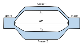
You are modeling the flow of water for a city. Two houses are connected in parallel to the main water supply, so that water from the main supply flows into either house 1 or house 2, and the flows out of each house then join up again at the main supply. The difference in pressure, \(∆P\), between the entry and exit point of water is the same for each house, and each house can be modeled as having a net resistance, \(R_{1}\) or \(R_{2}\), to the flow of water, as illustrated in Figure \(\PageIndex{10}\). If you model the two houses as being the equivalent of a single “effective” house with an effective resistance \(R\), what is the value of \(R\) in terms of \(R_{1}\) and \(R_{2}\)?
Solution
The water from the main will have to flow through either house 1 or house 2. If the flow rate through the main is \(Q\), we require that this be equal to the sum of the flow rates through each house:
\[\begin{aligned} Q=Q_{1}+Q_{2} \end{aligned}\]
The flow through each house is related to the pressure difference, \(∆P\), across each house (which is the same), as well as the resistance of that house:
\[\begin{aligned} Q_{1}&=\frac{\Delta P}{R_{1}} \\[4pt] Q_{2}&=\frac{\Delta P}{R_{2}} \end{aligned}\]
The total flow rate is thus:
\[\begin{aligned} Q=Q_{1}+Q_{2}&=\frac{\Delta P}{R_{1}}+\frac{\Delta P}{R_{2}} \\[4pt] &=\Delta P \left(\frac{1}{R_{1}}+\frac{1}{R_{2}}\right) \end{aligned}\]
We can write this as the flow through an effective resistance, \(R\), with a pressure difference \(∆P\):
\[\begin{aligned} Q&=\frac{\Delta P}{R} \\[4pt] \therefore R&=\frac{1}{\frac{1}{R_{1}}+\frac{1}{R_{2}}} \end{aligned}\]
Discussion
By requiring that the sum of the flows of water through the houses be the same as the flow rate through the main pipe, we were able to model the two houses as a single effective house with resistance \(R\). You may notice that this is the same relation as the equivalent resistance for two electrical resistors combined in parallel. This is because the flow of electrical current in a resistor can be modeled using similar tools to those required for modeling the flow of a viscous fluid in a pipe.
Footnotes
1. If the velocity of the fluid is not perpendicular to the surface, then \(v\) is the component of the velocity perpendicular to the surface.