
17.1: Flux of the Electric Field
- Page ID
- 19487
Gauss’ Law makes use of the concept of “flux”. Flux is always defined based on:
- A surface.
- A vector field (e.g. the electric field).
and can be thought of as a measure of the number of field lines from the vector field that cross the given surface. For that reason, one usually refers to the “flux of the electric field through a surface”. This is illustrated in Figure \(\PageIndex{1}\) for a uniform horizontal electric field, and a flat surface, whose normal vector, \(\vec A\), is shown. If the surface is perpendicular to the field (left panel), and the field vector is thus parallel to the vector, \(\vec A\), then the flux through that surface is maximal. If the surface is parallel to the field (right panel), then no field lines cross that surface, and the flux through that surface is zero. If the surface is rotated with respect to the electric field, as in the middle panel, then the flux through the surface is between zero and the maximal value.
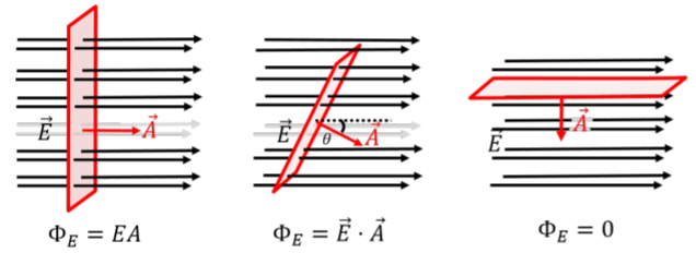
We define a vector, \(\vec A\), associated with the surface such that the magnitude of \(\vec A\) is equal to the area of the surface, and the direction of \(\vec A\) is such that it is perpendicular to the surface, as illustrated in Figure \(\PageIndex{1}\). We define the flux, \(\Phi_E\), of the electric field, \(\vec E\), through the surface represented by vector, \(\vec A\), as:
\[\begin{aligned} \Phi_E=\vec E\cdot \vec A=EA\cos\theta\end{aligned}\]
since this will have the same properties that we described above (e.g. no flux when \(\vec E\) and \(\vec A\) are perpendicular, flux proportional to number of field lines crossing the surface). Note that the flux is only defined up to an overall sign, as there are two possible choices for the direction of the vector \(\vec A\), since it is only required to be perpendicular to the surface. By convention, we usually choose \(\vec A\) so that the flux is positive.
What are the S.I. units of electric flux?
- \(\text{N}\cdot\text{m/C}\)
- \(\text{V}\cdot\text{m}\)
- \(\text{V/m}\)
- The units of flux depend on the dimensions of the charged object.
- Answer
-
The units of flux depend on the dimensions of the charged object.
A uniform electric field is given by: \(\vec E=E\cos\theta\hat x+E\sin\theta\hat y\) throughout space. A rectangular surface is defined by the four points \((0,0,0)\), \((0,0,H)\), \((L,0,0)\), \((L,0,H)\). What is the flux of the electric field through the surface?
Solution
The surface that is defined corresponds to a rectangle in the \(xz\) plane with area \(A=LH\). Since the rectangle lies in the \(xz\) plane, a vector perpendicular to the surface will be along the \(y\) direction. We choose the positive \(y\) direction, since this will give a positive number for the flux (as the electric field has a positive component in the \(y\) direction). The vector \(\vec A\) is given by:
\[\begin{aligned} \vec A =A\hat y=LH\hat y\end{aligned}\]
The flux through the surface is thus given by:
\[\begin{aligned} \Phi_E&=\vec E\cdot \vec A=(E\cos\theta\hat x+E\sin\theta\hat y)\cdot(LH\hat y)\\[4pt] &=ELH\sin\theta\end{aligned}\]
where one should note that the angle \(\theta\), in this case, is not the angle between \(\vec E\) and \(\vec A\), but rather the complement of that angle.
Discussion
In this example, we calculated the flux of a uniform electric field through a rectangle of area, \(A=LH\). Since we knew the components of both the electric field vector, \(\vec E\), and the surface vector, \(\vec A\), we used their scalar product to determine the flux through the surface. In some cases, it is easier to work with the magnitude of the vectors and the angle between them to determine the scalar product (although note that in this example, the angle between \(\vec E\) and \(\vec A\) is \(90^{\circ}-\theta\)).
Non-uniform fields
So far, we have considered the flux of a uniform electric field, \(\vec E\), through a surface, \(S\), described by a vector, \(\vec A\). In this case, the flux, \(\Phi_E\), is given by:
\[\begin{aligned} \Phi_E=\vec E\cdot \vec A\end{aligned}\]
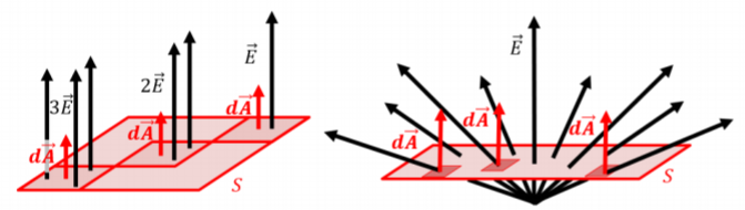
However, if the electric field is not constant in magnitude and/or in direction over the entire surface, then we divide the surface, \(S\), into many infinitesimal surfaces, \(dS\), and sum together (integrate) the fluxes from those infinitesimal surfaces:
\[\Phi_{E}=\int\vec E\cdot d\vec A\]
where, \(d\vec A\), is the normal vector for the infinitesimal surface, \(dS\). This is illustrated in Figure \(\PageIndex{2}\), which shows, in the left panel, a surface for which the electric field changes magnitude along the surface (as the field lines are closer in the lower left part of the surface), and, in the right panel, a scenario in which the direction and magnitude of the electric field vary along the surface.
In order to calculate the flux through the total surface, we first calculate the flux through an infinitesimal surface, \(dS\), over which we assume that \(\vec E\) is constant in magnitude and direction, and then, we sum (integrate) the fluxes from all of the infinitesimal surfaces together. Remember, the flux through a surface is related to the number of field lines that cross that surface; it thus makes sense to count the lines crossing an infinitesimal surface, \(dS\), and then adding those together over all the infinitesimal surfaces to determine the flux through the total surface, \(S\).
An electric field points in the \(z\) direction everywhere in space. The magnitude of the electric field depends linearly on the \(x\) position in space, so that the electric field vector is given by: \(\vec E=(a-bx)\hat z\), where, \(a\), and, \(b\), are constants. What is the flux of the electric field through a square of side, \(L\), that is located in the positive \(xy\) plane with one of its corners at the origin? We need to calculate the flux of the electric field through a square of side \(L\) in the \(xy\) plane. The electric field is always in the \(z\) direction, so the angle between \(\vec E\) and \(d\vec A\) (the normal vector for any infinitesimal area element) will remain constant.
Solution
We can calculate the flux through the square by dividing up the square into thin strips of length \(L\) in the \(y\) direction and infinitesimal width \(dx\) in the \(x\) direction, as illustrated in Figure \(\PageIndex{3}\). In this case, because the electric field does not change with \(y\), the dimension of the infinitesimal area element in the \(y\) direction is finite (\(L\)). If the electric field varied both as a function of \(x\) and \(y\), we would start with area elements that have infinitesimal dimensions in both the \(x\) and the \(y\) directions.
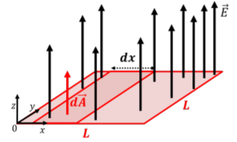
As illustrated in Figure \(\PageIndex{3}\), we first calculate the flux through a thin strip of area, \(dA=Ldx\), located at position \(x\) along the \(x\) axis. Choosing, \(d\vec A\), in the direction to give a positive flux, the flux through the strip that is illustrated is given by:
\[\begin{aligned} d\Phi_E=\vec E\cdot d\vec A=EdA=(ax-b)Ldx\end{aligned}\]
where \(\vec E\cdot d\vec A=EdA\), since the angle between \(\vec E\) and \(\vec A\) is zero. Summing together the fluxes from the strips, from \(x=0\) to \(x=L\), the total flux is given by:
\[\begin{aligned} \Phi_E=\int d\Phi_E=\int_0^L(ax-b)Ldx=\frac{1}{2}aL^3-bL^2\end{aligned}\]
Discussion
In this example, we showed how to calculate the flux from an electric field that changes magnitude with position. We modeled a square of side, \(L\), as being made of many thin strips of length, \(L\), and width, \(dx\). We then calculated the flux through each strip and added those together to obtain the total flux through the square.
Closed surfaces
One can distinguish between a “closed” surface and an “open” surface. A surface is closed if it completely defines a volume that could, for example, be filled with a liquid. A closed surface has a clear “inside” and an “outside”. For example, the surface of a sphere, of a cube, or of a cylinder are all examples of closed surfaces. A plane, a triangle, and a disk are, on the other hand, examples of “open surfaces”.
For a closed surface, one can unambiguously define the direction of the vector \(\vec A\) (or \(d\vec A\)) as the direction that it is perpendicular to the surface and points towards the outside. Thus, the sign of the flux out of a closed surface is meaningful. The flux will be positive if there is a net number of field lines exiting the volume defined by the surface (since \(\vec E\) and \(\vec A\) will be parallel on average) and the flux will be negative if there is a net number of field lines entering the volume (as \(\vec E\) and \(\vec A\) will be anti-parallel on average). The flux through a closed surface is thus zero if the number of field lines that enter the surface is the same as the number of field lines that exit the surface.
When calculating the flux over a closed surface, we use a different integration symbol to show that the surface is closed:
\[\begin{aligned} \Phi_E=\oint \vec E\cdot d\vec A\end{aligned}\]
which is the same integration symbol that we used for indicating a path integral when the initial and final points are the same (see for example Section 8.1).
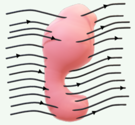
A non-uniform electric field \(\vec E\) flows through an irregularly-shaped closed surface, as shown in Figure \(\PageIndex{4}\). The flux through the surface is
- positive.
- zero.
- negative.
- Answer
A negative electric charge, \(-Q\), is located at the origin of a coordinate system. Calculate the flux of the electric field through a spherical surface of radius, \(R\), that is centerd at the origin.
Solution
Figure \(\PageIndex{5}\) shows the spherical surface of radius, \(R\), centerd on the origin where the charge \(-Q\) is located.
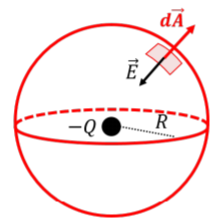
At all points along the surface, the electric field has the same magnitude:
\[\begin{aligned} E=\frac{1}{4\pi\epsilon_0}\frac{Q}{R^2}\end{aligned}\]
as given by Coulomb’s law for a point charge. Although the vector, \(\vec E\), changes direction everywhere along the surface, it always makes the same angle (-180) with the corresponding vector, \(d\vec A\), at any particular location. Indeed, for a point charge, the electric field points in the radial direction (inwards for a negative charge) and is thus perpendicular to the spherical surface at all points. Since the surface is closed, the vector, \(d\vec A\), points outwards anywhere on the surface. Thus, at any point on the surface, we can evaluate the flux through an infinitesimal area element, \(d\vec A\):
\[\begin{aligned} d\Phi_E=\vec E\cdot d\vec A=EdA\cos(-180^{\circ})=-EdA\end{aligned}\]
where the overall minus sign comes from the fact that, \(\vec E\), and, \(d\vec A\), are anti-parallel. The total flux through the spherical surface is obtained by summing together the fluxes through each area element:
\[\begin{aligned} \Phi_E=\oint d\Phi_E=\oint -EdA=-E\oint dA=-E(4\pi R^2)\end{aligned}\]
where we factored, \(E\), out of the integral, since the magnitude of the electric field is constant over the entire surface (a constant distance \(R\) from the charge). In the last equality, we recognized that, \(\oint dA\), simply means “sum together all of the areas, \(dA\), of the surface elements”, which gives the total surface area of the sphere, \(4\pi R^2\). The flux through the spherical surface is negative, because the charge is negative, and the field lines point towards \(-Q\).
Using the value that we obtained for the magnitude of the electric field from Coulomb’s Law, the total flux is given by:
\[\begin{aligned} \Phi_E=-E(4\pi R^2)=-\frac{1}{4\pi\epsilon_0}\frac{Q}{R^2}(4\pi R^2)=-\frac{Q}{\epsilon_0}\end{aligned}\]
which, surprisingly, is independent of the radius of the spherical surface. Note that we used \(\epsilon_0\) instead of Coulomb’s constant, \(k\), since the result is cleaner without the extra factor of \(4\pi\).
Discussion
In this example, we calculated the flux of the electric field from a negative point charge through a spherical surface concentric with the charge. We found the flux to be negative, which makes sense, since the field lines go towards a negative charge, and there is thus a net number of field lines entering the spherical surface. Perhaps surprisingly, we found that the total flux through the surface does not depend on the radius of the surface! In fact, that statement is precisely Gauss’ Law: the net flux out of a closed surface depends only on the amount of charge enclosed by that surface (and the constant, \(\epsilon_0\)). Gauss’ Law is of course more general, and applies to surfaces of any shape, as well as charges of any shape (whereas Coulomb’s Law only holds for point charges).