18.3: Calculating electric potential from charge distributions

In this section, we give two examples of determining the electric potential for different charge distributions. We have two methods that we can use to calculate the electric potential from a distribution of charges:

1. Model the charge distribution as the sum of infinitesimal point charges, \(dq\), and add together the electric potentials, \(dV\), from all charges, \(dq\). This requires that one choose \(0\text{V}\) to be located at infinity, so that the \(dV\) are all relative to the same point.
2. Calculate the electric field (either as a integral or from Gauss’ Law), and use:

   \[\begin{aligned} \Delta V &=V(\vec r_B)-V(\vec r_A)=-\int_A^B \vec E\cdot d\vec r\end{aligned}\]

The first method is similar to how we calculated the electric field for distributed charges in chapter 16, but with the simplification that we only need to sum scalars instead of vectors. The second method was already introduced in this chapter.

Example \(\PageIndex{1}\)

A ring of radius \(R\) carries a total charge \(+Q\). Determine the electric potential a distance \(a\) from the center of the ring, along the axis of symmetry of the ring. Assume that zero electric potential is defined at infinity.

Solution

Figure \(\PageIndex{1}\) shows a diagram of the ring, and our choice of infinitesimal charge, \(dq\).

Figure \(\PageIndex{1}\): Determining the electric potential on the axis of a ring of radius \(R\) carrying charge \(Q\).

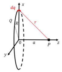
In order to calculate the electric potential at point, \(P\), with \(0\text{V}\) defined to be at infinity, we first calculate the infinitesimal potential at \(P\) from the infinitesimal point charge, \(dq\):

\[\begin{aligned} dV=k\frac{dq}{r}\end{aligned}\]

The total electric potential is then the sum (integral) of these potentials:

\[\begin{aligned} V=\int dV=\int k\frac{dq}{r} = \frac{k}{r}\int dq=k\frac{Q}{r}=k\frac{Q}{\sqrt{a^2+R^2}}\end{aligned}\]

where we recognized that \(k\) and \(r\) are the same for each \(dq\), so that they could factor out of the integral. \(\int dq=Q\) is then just the sum of the infinitesimal charges, which must add to the charge of the ring.

Discussion

In this example, we determined the electric potential, relative to infinity, a distance \(a\) from the center of a charge ring, along its axis of symmetry. We modeled the ring as being made of many infinitesimal point charges, and summed together the infinitesimal electric potentials from those charges relative to infinity. This was much simpler than determining the electric field, since electric potential is a scalar and we do not need to consider how the components from different \(dq\) along the ring will cancel.

Example \(\PageIndex{2}\)

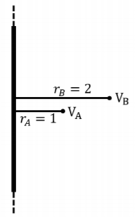
A long, thin, straight wire carries uniform charge per unit length, \(\lambda\). The electric potential difference between points located at distances \(r_B=2\text{cm}\) and \(r_A=1\text{cm}\) from the wire is found to be \(V(r_B)-V(r_A)=-100\text{V}\). What is the linear charge density on wire, \(\lambda\)?

Figure \(\PageIndex{2}\): A long thin wire with measurements of electric potential at varying points.

Solution

In this case, we can use Gauss’ Law to determine the electric field at a certain distance from the wire. From that, we can calculate the electric potential difference between any two points near the wire, and thus the charge density on the wire.

By using a cylindrical surface of length, \(L\), and radius, \(r\), we can use Gauss’ Law to determine the field at a distance, \(r\), from the wire:

\[\begin{aligned} \oint \vec E\cdot d\vec A&=\frac{Q^{enc}}{\epsilon_0}\\[4pt] 2\pi r L E&= \frac{\lambda L}{\epsilon_0}\\[4pt] \therefore \vec E(r)&=\frac{\lambda}{2\pi\epsilon_0 r}\hat r\end{aligned}\]

Using the electric field, we can calculate the potential difference between two points that are at distances, \(r_A\) and \(r_B\), from the wire:

\[\begin{aligned} \Delta V &=V(r_B)-V(r_A)=-\int_{r_A}^{r_B} \vec E\cdot d\vec r\\[4pt] &=-\int_{r_A}^{r_B} \left( \frac{\lambda}{2\pi\epsilon_0 r}\hat r \right)\cdot d\vec r=-\frac{\lambda}{2\pi\epsilon_0}\int_{r_A}^{r_B} \frac{1}{r}\hat r \cdot d\vec r=-\frac{\lambda}{2\pi\epsilon_0}\int_{r_A}^{r_B} \frac{1}{r}dr\\[4pt] &=-\frac{\lambda}{2\pi\epsilon_0}\left[|\ln(r)|\right]_{r_A}^{r_B} = -\frac{\lambda}{2\pi\epsilon_0}\ln\left(\frac{r_B}{r_A}\right)\\[4pt] \therefore\Delta V &=\frac{\lambda}{2\pi\epsilon_0}\ln\left(\frac{r_A}{r_B}\right)\end{aligned}\]

where, in the second last line, we removed the absolute value from the logarithm, since \(r_A<r_B\), and in the last line, we removed the minus sign by inverting the argument of the logarithm. Since we know the potential difference, \(\Delta V\), for two points located at distances \(r_B=2\text{cm}\) and \(r_A=1\text{cm}\), we can determine the charge density on the wire:

\[\begin{aligned} \Delta V &=V(r_B)-V(r_A)=-100\text{V}\\[4pt] \Delta V &=\frac{\lambda}{2\pi\epsilon_0}\ln\left(\frac{r_A}{r_B}\right)\\[4pt] \therefore \lambda &= \frac{2\pi\epsilon_0\Delta V}{\ln\left(\frac{r_A}{r_B}\right)}=\frac{2\pi(8.85\times 10^{-12}\text{C}^2\cdot \text{N}^{-1}\cdot \text{m}^{-2})(-100\text{V})}{\ln\left(\frac{1}{2}\right)}=8.02\times 10^{-9}\text{C/m}\end{aligned}\]

where, again, one needs to be very careful with the signs! Note that it also makes sense that the potential difference, \(\Delta V =V(r_B)-V(r_A)\), is negative, since \(r_A\) is closer to the positively charged wire. A positive charge at rest would move away from the positively charged wire, from \(r_A\) to \(r_B\), from high potential to low potential.

Discussion

In this example, we showed how to determine the electric potential near an infinitely long charged wire by using the electric field that we determined from Gauss’ Law. By knowing the potential difference between two points near the wire, we were then able to infer the charge density on the wire.