19.1: Current

In the preceding chapters, we examined “electrostatic” systems; those for which charges are not in motion. In electrostatic systems, the electric field inside of a conductor is zero (by definition, or charges would be moving, since they are free to move in a conductor). We argued that if charges are deposited onto a conductor, they would quickly arrange themselves into a static configuration (on the surface of the conductor).

Instead, we can build systems were charges move in a conductor. If we apply a fixed potential difference across a conductor, this will result in an electric field inside the conductor and the charges within will move as a result. In general, this requires that there be some sort of circuit formed, whereby charges enter one end of the conductor and exit the other. The most simple circuit that one can construct is to connect the two terminals of a battery to the ends of a conductor, as illustrated in Figure \(\PageIndex{1}\).

Figure \(\PageIndex{1}\): A simple circuit is created by connecting the terminals of a battery to a conducting material such as a copper wire. Note that while electrons flow from the negative to the positive terminal of the battery, conventional current is defined as if it were positive charges moving in the opposite direction.

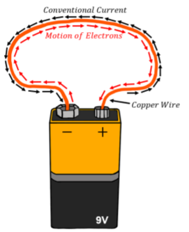
A battery (as we will see in more detail in Section 20) is a device that provides a source of charges and a fixed potential difference. For example, a \(9\text{V}\) battery has two terminals with a constant voltage of \(9\text{V}\) between them.

“Electric current” is defined to be the rate at which charges cross a given plane (usually a plane perpendicular to some conductor through which we want to define the current). We define current, \(I\), as the total amount of charge, \(\Delta Q\), that flows through any cross-section of the conductor during an amount of time, \(\Delta t\):

\[I=\frac{\Delta Q}{\delta t}=\frac{dQ}{dt}\]

where we take a derivative if the rate at which charges flow is not constant in time. The S.I. unit of current is the Ampère (A). Current is defined to be positive in the direction in which positive charges flow. In almost all cases, it is negative electrons that flow through a material; the current is defined to be in the opposite direction from which the actual electrons are flowing, as illustrated in Figure \(\PageIndex{1}\). To distinguish that the current is in the direction opposite to that of the flowing electrons, one sometimes uses the term “conventional current” to indicate that the current is referring to a flow of positive charges.

Note that the definition of electric current is very similar to the “flow rate”, \(Q\), that we defined as the volume flow of a liquid across a given cross-section (Section 15.3). As we continue to develop our description of current, you will notice that there are many similarities between describing the flow of an incompressible fluid and describing the flow of charges in a conductor.

We think of current as a macroscopic quantity, something that we can easily measure in the lab. Current is a measure of the average rate at which charges are moving through the conductor, and not a measure of what is going on at a microscopic level. In order to model the motion of charges at the microscopic level, we introduce the “current density”, \(\vec j\):

\[\vec j =\frac{I}{A}\hat E\]

where, \(I\), is the current that flows through a surface with cross-sectional area, \(A\), and \(\hat E\) is a unit vector in the direction of the electric field at the point where we are determining the current density. The current density allows us to develop a microscopic description of the current, since it is the electric current per unit area and points in the direction of the electric field at some position. Given the current density, \(\vec j\), one can always determine the current through a surface with area, \(A\), and normal vector, \(\hat n\):

\[\begin{aligned} I = A(\vec j\cdot \hat n)\end{aligned}\]

If the current density changes over the surface, one must take an integral instead:

\[\begin{aligned} I=\int \vec j \cdot d\vec A\end{aligned}\]

where \(d\vec A\), is a surface element with area, \(A\), and direction given by the normal to the surface at that point. The overall sign of the current will be determined by the direction of the flow of positive charges.

Example \(\PageIndex{1}\)

Electric current flows through a conductor with a narrowing cross section, as illustrated in Figure \(\PageIndex{2}\). If the cross-sectional area the conductor is \(A_1\) at one end, and \(A_2\), at the other end, what is the ratio of the current densities, \(j_1/j_2\), at the two ends of the conductor?

Solution

Figure \(\PageIndex{2}\): Current flows through a conductor with a cross-section that decreases from \(A_{1}\) to \(A_{2}\).

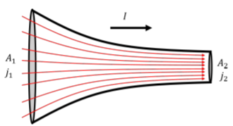
This situation is very similar to the flow of an incompressible fluid. In this case, the number of charges entering the conductor must be equal to the number of charges exiting the conductor during a given amount of time. That is, the total current, \(I\), must be the same at both ends, since there is no place in the conductor for charges to accumulate. Since the current must be the same on both ends, we can relate the current densities at each end:

\[\begin{aligned} j&=\frac{I}{A}\\[4pt] \therefore I&=j_1A_1=j_2A_2\\[4pt] \therefore \frac{j_2}{j_1}&=\frac{A_1}{A_2}\end{aligned}\]

and we find that the current density at the exit of the conductor must be higher than at the entrance. This is similar to the continuity equation in the Fluid Mechanics chapter (Section 15.3), where the current density plays a role analogous to the velocity in the fluids case.