
19.2: Microscopic model of current
- Page ID
- 19505
Consider a cylindrical conductor of cross-sectional area, \(A\), and length, \(L\), as shown in Figure \(\PageIndex{1}\). A potential difference, \(\Delta V\), is applied across the length of the conductor, so that there is an electric field, \(\vec E\), everywhere within the conductor. If the conductor were made of empty space, electrons would enter one end of the conductor, accelerate through the potential difference, and arrive at the other end with a high speed, having gained \(e\Delta V\) of kinetic energy. In reality, the conductor is made of matter, and electrons do not accelerate continuously through the whole length of the conductor. Instead, they can only accelerate over a short distance before colliding with an atom in the material (rather, a tightly bound electron in the material), and losing their kinetic energy to the material, before accelerating again. The motion of electrons flowing in a conductor is illustrated in Figure \(\PageIndex{1}\) and shows electrons moving with a wide range of velocities following the collisions, and only an average motion in the direction anti-parallel to the electric field.
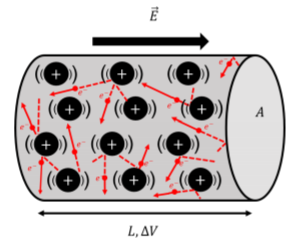
Thus, when the electrons arrive at the positive side of the conductor, they have not gained any kinetic energy. Instead, they have lost that kinetic energy to atoms of the conducting material through collisions; those atoms then vibrate which we can measure as an increase in temperature of the material. When current flows through a conductor, that conductor will heat up; this is how the heating elements in your toaster work!
We model the motion of electrons as charges “drifting” through the conductor with a velocity, \(\vec v_d\), the “drift velocity”, as illustrated in Figure \(\PageIndex{2}\). In reality, of course, the electrons are only moving on average with the drift velocity, and their instantaneous speed is generally much larger than the drift velocity and can be in any direction, as illustrated in Figure \(\PageIndex{1}\).
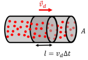
In a conducting material, each atom will generally have one “free” electron that is loosely bound and able to easily move through the material. The number of free electrons available for conduction per unit volume, \(n\), will depend properties of the material (its density, how many electrons per atom are available, etc). Consider, then, the motion of the conduction electrons present in a section of length, \(l\), of a conductor, as illustrated in Figure \(\PageIndex{2}\). The amount of charge, \(\Delta Q\), contained in a section of the conductor with length, \(l\), is given by:
\[\begin{aligned} \Delta Q= -e n Al\end{aligned}\]
where \(Al\) is the volume of that section of the conductor, and, \(e\), is the magnitude of the charge of the electron. The negative sign is to indicate that the charges are negative (they are electrons). That charge will take an amount of time, \(\Delta t\), to flow through a given plane of the conductor, so that we can relate the length of the section, \(l\), to the drift speed and \(\Delta t\):
\[\begin{aligned} l&=v_d\Delta t\end{aligned}\]
Thus, the current that flows through a cross-section of the conductor is given by:
\[\begin{aligned} I =\frac{\Delta Q}{\delta t}=\frac{-enAl}{\Delta t}=-enAv_{d} \end{aligned}\]
\[\therefore I=-enAv_{d}\]
which allows us to connect a macroscopic quantity, current, to the microscopic description of charges moving. Note that the negative sign reflects the fact that the current (of positive charges) is in the opposite direction from the drift velocity of the (negative) electrons. The current density is directly related to the microscopic quantities, since it does not depend on the (macroscopic) cross-sectional area, \(A\), of the conductor:
\[\begin{aligned} \vec j=\frac{I}{A}\hat E=-en\vec v_{d} \end{aligned}\]
\[\therefore \vec j=-en\vec v_{d}\]
where, again, the negative sign indicates that the current density is in the opposite direction from the actual drift velocity of the electrons, which itself is anti-parallel to the electric field.
A current of \(1\text{A}\) is measured in a copper wire with a diameter of \(1\text{mm}\). What is the drift velocity of the electrons? Assume that each atom of copper provides one “free electron” for conduction.
Solution
In order to determine the drift velocity of electrons, we need to know the density of free electrons in copper. To do this, we need to determine how many copper atoms there are per unit volume. The density of copper is \(\rho=8.92\times 10^{3}\text{kg/m}^{3}\) and the atomic mass unit of copper is \(63.5\text{amu}\) (\(1\text{mole}\) of copper weighs \(63.5\text{g}\)). The number of copper atoms per unit volume is thus:
\[\begin{aligned} n=\frac{(6.022\times 10^{23}\text{mole}^{-1})(8.92\times 10^{3}\text{kg/m}^{3})}{(63.5\times 10^{-3}\text{kg/mole})}=8.46\times 10^{28}\text{m}^{-3}\end{aligned}\]
Since each copper atom contributes one free electron, this is the same as the density of free electrons. From this, we easily obtain the drift velocity, from the current:
\[\begin{aligned} v_d&=\frac{j}{en}=\frac{I}{Aen}=\frac{(1\text{A})}{\pi(0.0005\text{m})^2(1.6\times 10^{-19}\text{C})(8.46\times 10^{28}\text{m}^{-3})}\\[4pt] &=9.4\times 10^{-5}\text{m/s}\sim 0.1\text{mm/s}\end{aligned}\]
The drift velocity is thus very slow, less than one millimetre per second. Note that a \(1\text{mm}\) diameter copper wire would not actually be able to sustain such a high current density without damage.
There are a few types of velocities which can be easily confused when discussing current: Fermi velocity, drift velocity, and the velocity at which a circuit is “completed”.
Understanding the Fermi velocity requires quantum mechanics and is beyond the scope of this textbook. However, the Fermi velocity is representative of the actual velocity of electrons in a conducting material, mostly due to their thermal energy. In a good conductor, these speed are roughly 1/200 the speed of light.
While electrons do move at their Fermi velocity in a conductor, they do not move in a uniform path through the conductor towards the end of the circuit. Most of an electron’s movement in a wire is chaotic, but in a DC circuit, the electrons have a drift velocity through the conductor. This drift velocity is defined as the net velocity of electrons in a conductor, and is caused by the applied electric field which has a small amount of influence on the direction of the quickly moving electron’s motion. The drift velocity of electrons is very slow, often having a magnitude as small as tens of microns per second.
When comparing drift velocity to Fermi speed, imagine yourself standing inside of a large horizontal cylinder, which will represent the conductor in this analogy. The interior of this cylinder is lined with cannons that shoot rubber balls in all directions, which will be the electrons moving at their Fermi velocity. Now, imagine that you are attempting to move these high-speed rubber balls from one end of the cylinder to the other by blowing a hair dryer in that direction, which is the electric field inducing a drift velocity.
Now that we understand the quantum chaos that occurs in a conductor, you may be thinking to yourself, "why does the light bulb turn on so quickly after I flick the light switch?". This is a reasonable thought, because we have only covered the motion of single particles in a conductor. When an electron moves very slightly (at its drift velocity), it will push other electrons in the conductor forward, causing a chain reaction of electrons pushing one another forward. This movement causes electrons to flow through the circuit, much like how water flows through a pipe. The velocity at which a light bulb turns on after the flicking of a switch is theoretically the speed of light, but short delays caused by irregularities in the way electrons bump into one another causes the velocity to be roughly 50 to 99 percent of the speed of light.