
22.3: Ampere’s Law
- Page ID
- 19535
Ampere’s Law is similar to Gauss’ Law, as it allows us to (analytically) determine the magnetic field that is produced by an electric current in configurations that have a high degree of symmetry. Ampere’s Law states:
\[\oint\vec B\cdot d\vec l=\mu_{0}I^{enc}\]
where the integral on the left is a “path integral”, similar to how we calculate the work done by a force over a particular path. The circle sign on the integral means that this is an integral over a “closed” path; a path where the starting and ending points are the same. \(I^{enc}\) is the net current that crosses the surface that is defined by the closed path, often called the “current enclosed” by the path. This is different from Gauss’ Law, where the integral is over a closed surface (not a closed path, as it is here). In the context of Gauss’ Law, we refer to “calculating the flux of the electric field through a closed surface”; in the context of Ampere’s Law, we refer to “calculating the circulation of the magnetic field along a closed path”.
We apply Ampere’s Law in much the same way as we apply Gauss’ Law.
- Make a good diagram, identify symmetries.
- Choose a closed path over which to calculate the circulation of the magnetic field (see below for how to choose the path). The path is often called an “Amperian loop” (think “Gaussian surface”).
- Evaluate the circulation integral.
- Determine how much current is “enclosed” by the Amperian loop.
- Apply Ampere’s Law.
Similarly to Gauss’ Law, we need to choose the path (instead of the surface) over which we will evaluate the integral. The integral will be easy to evaluate if:
1. The angle between \(\vec B\) and \(d\vec l\) is constant along the path, so that:
\[\begin{aligned} \oint\vec B\cdot d\vec l=\oint Bdl\cos\theta=\cos\theta\oint Bdl \end{aligned}\]
where \(\theta\) is the angle between \(\vec B\) and \(d\vec l\).
2. The magnitude of \(\vec B\) is constant along the path, so that:
\[\begin{aligned} \cos\theta\oint Bdl=B\cos\theta\oint dl \end{aligned}\]
Choosing a path that meets these two conditions is only possible if there is a high degree of symmetry.
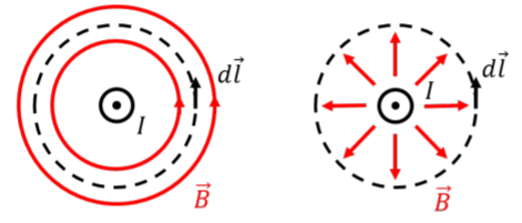
Consider an infinitely long straight wire, carrying current, \(I\), out of the page, as illustrated in Figure \(\PageIndex{1}\). The magnetic field from the wire must look the same regardless of the angle from which we view the wire (“azimuthal symmetry”). Thus, the magnetic field must either form concentric circles around the wire (which we know is the case from the Biot-Savart Law) or it must be in the radial direction (pointing towards or away from the wire). These two possibilities are illustrated in Figure \(\PageIndex{1}\), and we will pretend, for now, that we do not know which is correct.
In order to apply Amp`ere’s Law, we choose an Amperian loop (instead of a “Gaussian surface”). In the case of an infinite current-carrying wire, a circle that is concentric with the wire will meet the properties above, regardless of the two possible configurations of the magnetic field: with a circular Amperian loop, the angle between the magnetic field and the element \(d\vec l\) is constant along the entire loop, and the magnitude of the magnetic field is constant along the loop. Our choice of loop is illustrated in Figure \(\PageIndex{2}\), where we have illustrated the magnetic field for the case where it forms concentric circles.
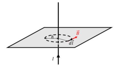
The circulation of the magnetic field along a circular path of radius, \(h\), is given by:
\[\begin{aligned} \oint\vec B\cdot d\vec l=\oint Bdl\cos\theta =\cos\theta\oint Bdl=B\cos\theta\oint dl=B\cos\theta (2\pi h) \end{aligned}\]
where \(\cos θ\) is \(1\) if the field forms circles (correct) or \(0\) if the field is radial (incorrect). We can now evaluate the current that is enclosed by the Amperian loop. The current that is enclosed is given by the net current that traverses the surface defined by the Amperian loop (in this case, a circle of radius \(h\)). Since the loop encloses the entire wire, the enclosed current is simply, \(I\). Applying Ampere’s Law:
\[\begin{aligned} \oint\vec B\cdot d\vec l&=\mu_{0}I^{enc} \\[4pt] B\cos\theta (2\pi h)&=\mu_{0}I \end{aligned}\]
At this point, it is clear that cos θ cannot be zero, since the right-hand side of the equation is not zero. We can thus conclude that the magnetic field must indeed make concentric circles, as we had previously determined. The magnitude of the magnetic field is given by:
\[\begin{aligned} B=\frac{\mu_{0}I}{2\pi h} \end{aligned}\]
as we found previously with the Biot-Savart Law. Again, in analogy with Gauss’ Law, one needs to apply some knowledge of symmetry and argue in which direction the magnetic field should point, in order to use Ampere’s Law effectively.
Ampere’s law proves that the magnetic field at the center of a current-carrying loop is zero because there is no enclosed current:
- True.
- False
- Answer
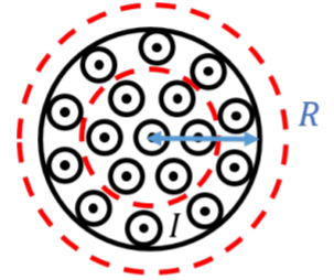
A long solid uniform cable of radius, \(R\), carries current, \(I\), with a current density that is uniform through the cross-section of the cable. Determine the strength of the magnetic field as a function of, \(r\), the distance from the center of the cable, inside and outside of the cable.
Solution
In this case, we need to determine the magnetic field both inside and outside of the cable. Figure \(\PageIndex{3}\) shows two circular Amperian loops that we can use to apply Ampere’s Law to determine the magnetic field inside and outside of the cable.
By symmetry, and following the discussion in this chapter, we know that the magnetic field must form concentric circles, both inside and outside of the cable. Outside the cable, we proceed in the same fashion as above, choosing an Amperian loop of radius, \(r > R\), such that the circulation is given by:
\[\begin{aligned} \oint\vec B\cdot d\vec l=B2\pi r \end{aligned}\]
The entire cable is enclosed by the loop, so that the enclosed current is, \(I\). Thus, Ampere’s Law gives:
\[\begin{aligned} \oint\vec B\cdot d\vec l&=\mu_{0}I^{enc} \\[4pt] B(2\pi r)&=\mu_{0}I \\[4pt] \therefore B&=\frac{\mu_{0}I}{2\pi r}\quad(r\geq R) \end{aligned}\]
Inside of the cable, the circulation integral around a circular path of radius, \(r < R\), is the same:
\[\begin{aligned} \oint\vec B\cdot d\vec l=B2\pi r \end{aligned}\]
However, in this case, the smaller Amperian loop does not enclose all of the current flowing through the cable. We are told that the current density, \(j\), is uniform in the cable. We can thus determine the current per unit area (i.e. the current density) that flows through the whole cable, and use that to determine how much current flows through the surface with area \(πr^{2}\) that is defined by the Amperian loop:
\[\begin{aligned} j&=\frac{I}{A}=\frac{I}{\pi R^{2}} \\[4pt] \therefore I^{enc}&=j(\pi r^{2})=\frac{I}{\pi R^{2}}(\pi r^{2})=I\frac{r^{2}}{R^{2}} \end{aligned}\]
Finally, we can apply Amp`ere’s Law to determine the magnitude of the magnetic field inside the cable:
\[\begin{aligned} \oint\vec B\cdot d\vec l&=\mu_{0}I^{enc} \\[4pt] B(2\pi r)&=\mu_{0}I\frac{r^{2}}{R^{2}} \\[4pt] \therefore B&=\frac{\mu_{0}I}{2\pi R^{2}}r \end{aligned}\]
and we find that the magnetic field is zero at the center of the cable (r = 0), and increases linearly up to the edge of the cable \((r = R)\).
Discussion
In this example, we used Ampere’s Law to model the strength of the magnetic field inside and outside of a current-carrying cable. In order to apply Ampere’s Law inside the cable, we took into account that only a fraction of the current is enclosed by the Amperian loop. This problem is analoguous to applying Gauss’ Law to determine the electric field inside and outside of a uniformly charged sphere.
Interpretation of Ampere's Law and vector calculus
In this section, we discuss Amp`ere’s Law in the context of vector calculus and provide a different perspective, mostly for informational purposes. The integral that appears in Ampere’s Law is called the “circulation” of the vector field, \(\vec B\):
\[\begin{aligned} \oint\vec B\cdot d\vec l \end{aligned}\]
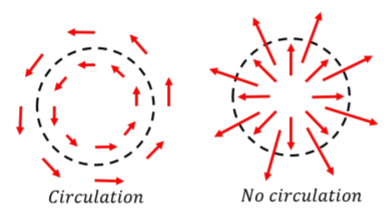
The circulation, as its name implies, is a measure of “how much rotation there is in the field”. To visualize this, imagine that the vector field is a velocity field for points in a fluid. Regions of the fluid where there are little whirlpools (so called “eddies”), correspond to regions of the field with non-zero circulation (the sign of the integral tells us the direction of rotation, using the right-hand rule for axial vectors). Examples of field with and without circulation are shown in Figure \(\PageIndex{4}\). You will recognize that static electric charges create electric fields with no circulation (right panel), whereas static currents create magnetic fields with circulation.
Ampere’s Law is thus a statement that an electric current will result in a field with a magnitude proportional to the current, that has some degree of rotation to it. The direction of rotation of that field corresponds to the right-hand rule for axial vectors as applied to the current (your thumb points in the direction of the current so that your fingers curl in the direction of the rotation of the associated field).
Circulation, as defined by the integral over a closed loop, is not a local property of the field, since it depends on what the field is doing as a whole over the path of the loop. Just as one can obtain a “local” version of Gauss’ Law, one can also obtain a local version of Amp`ere’s Law using techniques from advanced vector calculus (that are beyond the scope of this textbook).
Stokes’ theorem allows one to convert the circulation integral (a path integral on a closed loop) into a integral over the (open) surface that is defined by the loop:
\[\begin{aligned} \oint_{C}\vec Bd\vec l=\int_{S}(\nabla\times\vec B)\cdot d\vec A \end{aligned}\]
where the subscript \(C\) indicates that the integral is over a one-dimensional path, whereas the subscript \(S\) indicates that the integral is over a two-dimensional surface. The term, \(∇ × \vec B\), is called the “curl” of the magnetic field and is a local measure of the amount of rotation in the field. Applying Stokes’ theorem to Ampere’s Law yield:
\[\begin{aligned} \oint\vec B\cdot d\vec l&=\mu_{0}I^{enc} \\[4pt] \int_{S}(\nabla\times\vec B)\cdot d\vec A=\mu_{0}I^{enc} \end{aligned}\]
Note that we can also write the current, \(I^{enc}\), that is enclosed by the loop as the integral of the current density, \(\vec j\), over the surface defined by the loop:
\[\begin{aligned} I^{enc}=\int_{S}\vec j\cdot d\vec A \end{aligned}\]
Thus, we can write Ampere’s Law with integrals over the same surface on either side of the equation, implying that the integrands must be the same:
\[\begin{aligned} \int_{S}(\nabla\times\vec B)\cdot d\vec A=\mu_{0}\int_{S}\vec j\cdot d\vec A \end{aligned}\]
\[\therefore\nabla\times\vec B=\mu_{0}\vec j\]
This last equation now relates a local property (current density) to the magnetic field at that point, and is the usual form in which Ampere’s Law is presented (the so-called “differential form”, rather than the “integral form”).
The curl of the magnetic field, \(∇ × \vec B\), is a vector that is given by the following:
\[\begin{aligned} \nabla\times\vec B=\left(\frac{\partial B_{z}}{\partial y}-\frac{\partial B_{y}}{\partial z} \right)\hat x+\left(\frac{\partial B_{x}}{\partial z}-\frac{\partial B_{z}}{\partial x} \right)\hat y +\left( \frac{\partial B_{y}}{\partial x}-\frac{\partial B_{x}}{\partial y} \right)\hat z \end{aligned}\]
and the name “curl” is chosen because this is a measure of the amount of rotation (curl) in the field. In differential form, Ampere’s Law can read as: “a current density will create a (magnetic) field that has non-zero curl”.
Since Ampere’s Law in differential form is a vector equation (both sides are vectors), it really corresponds to three equations in Cartesian coordinates, one per component. For example, the \(x\) component of the equation is a “partial differential equation” for the \(y\) and \(z\) components of the magnetic field:
\[\begin{aligned} \left(\frac{\partial B_{z}}{\partial y}-\frac{\partial B_{y}}{\partial z} \right)=\mu_{0}j_{x} \end{aligned}\]
that is in general difficult to solve without a computer (and all three equations are required, as these are “coupled”, since a given component of the magnetic field appears in two of three equations).