24.1: Introduction- The issue with Maxwell’s equations

In Chapter 23, we summarized our knowledge of electromagnetism using Maxwell’s four equations. As far as we can tell, this is the best description that we have of classical electric and magnetic phenomena (classical in the sense that the equations do not describe the behaviour of particles that are described by Quantum Mechanics). One of the consequences of Maxwell’s equations is that they describe the existence of electromagnetic waves that propagate with a speed, \(c\), given by:

\[\begin{aligned} c = \frac{1}{\sqrt{\epsilon_0\mu_0}}\end{aligned}\]

where \(\epsilon_0\) and \(\mu_0\) are the permittivity and permeability of free-space, respectively. The obvious question to ask about these electromagnetic waves is: “In what medium do these waves propagate?”. In the late 1800s, it was thought that the Universe was bathed in a substance called the “luminous ether” (or just “ether”), through which electromagnetic waves propagate. It was then thought that the speed, \(c\), of these waves was, naturally, measured with respect to the ether. This led to the idea that there exists a special inertial frame of reference in the Universe, corresponding to that frame of reference in which light travels at a speed, \(c\). This frame of reference would be at rest relative to the ether.

In the late 1880s, Michelson and Morley developed a clever experiment to measure the speed of the Earth relative to the ether. If the ether exists, and the Earth is moving through it, then a beam of light travelling parallel to the motion of the Earth should travel at a slightly different speed than a beam of light travelling in the perpendicular direction. However, Michelson and Morley conclusively demonstrated that this was not the case. There is no detectable motion of the Earth through a medium in which light (a electromagnetic wave) propagates. There is no ether. This was a very puzzling discovery, with strange implications for Maxwell’s equations.

Let us demonstrate, through a simple example, an “issue” with the theory of electromagnetism. Rather, it is not an issue, but a very strange implication. Consider two infinitely-long wires, separated by a distance, \(r\), each carrying a uniform charge per unit length, \(\lambda\), as illustrated in Figure \(\PageIndex{1}\).

Figure \(\PageIndex{1}\): Two infinitely long charged wires exert a repulsive electric force on each other.

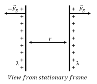
We can easily calculate the magnitude of the repulsive electric force, \(\vec F_E\), exerted by one charged wire on a section of length, \(l\), of the other wire. The magnitude of the electric field at a distance, \(r\), from an infinitely-long wire with charge per unit length, \(\lambda\), is given by:

\[\begin{aligned} E = \frac{\lambda}{2\pi \epsilon_0r}\end{aligned}\]

A section of length, \(l\), of the other wire carries charge, \(q=l\lambda\), so that the force on that section of wire has a magnitude:

\[\begin{aligned} F_E=qE=\lambda l \left( \frac{\lambda}{2\pi \epsilon_0r}\right) = \frac{\lambda^2 l}{2\pi \epsilon_0r}\end{aligned}\]

And the force per unit length, on either one of the wires, has a magnitude:

\[\begin{aligned} \frac{F_E}{l}=\frac{\lambda^2}{2\pi \epsilon_0r}\end{aligned}\]

This is the only force exerted on one of the wires, and will thus allow us to completely specify the motion of that wire (we know all of the forces exerted on the wire, so we can use Newton’s Second Law to determine its acceleration and describe its motion).

Consider the same two wires, each carrying charge per unit length but as viewed from a frame of reference that is moving downwards (parallel to the wires), with a speed, \(v\). In this frame of reference, the infinite wires still have a net charge per unit length, but they also appear to have an upwards moving current, \(I\), since we observe positive charges moving upwards through space.

Figure \(\PageIndex{2}\): Two infinitely-long charged wires as viewed from a down-going frame of reference will appear to have upwards-going currents that will result in an attractive magnetic force between the wires.

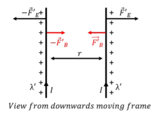
In this new frame of reference, we see two wires with charges on them, moving upwards with speed, \(v\). In a length of time, \(\Delta t\), we see a length of wire, \(\Delta x=v\Delta t\), go by, with total charge, \(\Delta Q=\lambda' \Delta x\). For reasons that will be clear below, we use a different charge density, \(\lambda'\), in the moving frame of reference, although we expect that \(\lambda'=\lambda\). This corresponds to a current, \(I\), given by:

\[\begin{aligned} I=\frac{\Delta Q}{\Delta t}=\lambda'\frac{\Delta x}{\Delta t}=\lambda' v\end{aligned}\]

Thus, in the downward going frame of reference, we see two wires with upwards current in them, and these wires must extract an attractive magnetic force between each other, with magnitude (per unit length):

\[\begin{aligned} \frac{F'_B}{l} = -\frac{\mu_0 I_1I_2}{2\pi r}=-\frac{\mu_0 I^2}{2\pi r}=-\frac{\mu_0 \lambda'^2 v^2}{2\pi r}\end{aligned}\]

where the prime (’) on the force indicates that the force is measured in this different inertial frame of reference, and the minus sign indicates that it is in the opposite direction from the repulsive electric force.

In the downwards going frame of reference, the wires are still charged, and must still exert a repulsive force, with magnitude (per unit length):

\[\begin{aligned} \frac{F'_E}{l}=\frac{\lambda'^2}{2\pi \epsilon_0r}\end{aligned}\]

where, again, we used primes (’), to denote quantities that are measured in the moving frame of reference.

The description of how the wires will move should not depend on the frame of reference that we choose to model the wires (they will move under the forces exerted on them regardless of whether we are observing them from a fixed or a moving point, and indeed regardless of whether we observe them at all!). Thus, the net force (per unit length) exerted on a wire cannot depend on our frame of reference. The total repulsive electric force, \(F_E\), calculated in the stationary frame of reference must be equal to the sum of the magnetic, \(F'_B\), and electric force, \(F'_E\), calculated in the moving frame of reference¹:

\[\begin{aligned} \frac{F_E}{l}&=\frac{F'_E}{l}+\frac{F'_B}{l}\\[4pt] \frac{\lambda^2}{2\pi \epsilon_0r}&=\frac{\lambda'^2}{2\pi \epsilon_0r} -\frac{\mu_0 \lambda'^2 v^2}{2\pi r}\end{aligned}\]

where we recognized that the charge per unit length, \(\lambda'\), must be different in the moving frame of reference, or the above would give an inconsistent equation (the electric forces would cancel and we would find that the magnetic force is equal to zero). Thus, the repulsive electric force must be larger as observed in the moving frame of reference, or the net force on the wire would be different when evaluated in the two frames of reference. This is a truly bizarre conclusion, as we will see.

Before proceeding, let us clearly state our assumptions in modeling the force between the two charged wires:

1. The net force on the wire, allowing us to describe its motion, cannot depend on our frame of reference. We expect the laws of physics to be applicable from any inertial frame of reference.
2. We assume that Maxwell’s equations hold in all inertial frames of reference. In particular, we assume that the constants, \(\mu_0\) and \(\epsilon_0\), are the same in all inertial reference frames.

The first assumption allows us to state that the net force in the two frames of reference must be the same. The second assumption implies that we must change the charge density, \(\lambda'\), in the moving frame of reference, since the constants must remain the same, and this is the only quantity that can lead to a different electric force in the moving frame of reference (which is required if the net force is to be the same, according to our first assumption). Let us determine the new charge density, \(\lambda'\), in terms of the charge density that is measured at rest. Starting with the requirement that the net force on the wire must not depend on the frame of reference, we find:

\[\begin{aligned} \frac{\lambda^2}{2\pi \epsilon_0r}&=\frac{\lambda'^2}{2\pi \epsilon_0r} -\frac{\mu_0 \lambda'^2 v^2}{2\pi r}\\[4pt] \lambda^2&=\lambda'^2-\epsilon_0\mu_0\lambda'^2 v^2\\[4pt] \lambda^2&=\lambda'^2(1-\epsilon_0\mu_0v^2)\\[4pt] \therefore \lambda'&=\lambda \frac{1}{\sqrt{\epsilon_0\mu_0-v^2}}\end{aligned}\]

Finally, recognizing that we can use the speed of light, \(c\), to replace the combination of constants, \(\epsilon_0\mu_0\), we find:

\[\begin{aligned} \lambda'&=\lambda \frac{1}{\sqrt{1-\frac{v^2}{c^2}}}\end{aligned}\]

Thus, the charge per unit length on the wire is larger when measured from the moving frame of reference (the factor that multiplies, \(\lambda\), is larger than one if \(v<c\)). It should be somewhat bothersome to you that the charge per unit length depends on the frame of reference in which it is measured, but this is the only way for our two assumptions to hold.

So far, this has just been some math to ensure that “things work out”, namely that our description of the motion of the wire does not depend on our frame of reference. However, the consequences of what we just derived are profound. We concluded that the charge per unit length on a wire depends on our frame of reference.

Imagine drawing two lines on one of the wires, and imagine that you can actually see the charges on the wire (maybe they fluoresce or something). The charge per unit length on the wire, \(\lambda\), is found by counting the number of charges between the two lines and dividing that by the distance between the two lines. Now, both an observer at rest with the wire, and one that is moving relative to the wire will agree on the number of charges contained between the two lines. They will both count the same number. Thus, if the observer moving relative to the wire is to measure a larger charge density, then the distance between the lines must be smaller for that observer! To the observer moving relative to the wire, the wire is actually shorter. It does not appear to be shorter, it IS shorter!

To summarize, by requiring that the laws of physics are the same in all inertial frames of reference, and by requiring that Maxwell’s equation are the same in all inertial frames of reference, we conclude that the charge per unit length that is measured on a wire must depend on the frame of reference in which it is measured. Since it cannot be the number of charges on the wire that depends on the frame of reference, it must be the length of the wire that depends on the frame of reference. Thus, either we accept that Maxwell’s equations are incorrect, or we accept that they are correct but that they imply that objects shrink in length when they are moving (regardless of whether charges are involved). It turns out that the latter choice provides a better description of nature (and one that has not been invalidated!).

As an additional consequence of accepting these implications from Maxwell’s equations is that the definition of the electric and magnetic fields must depend on the frame of reference. In the example from this section, we saw that what looks like an electric field in the stationary frame of reference, can appear as the combination of a magnetic and electric fields in a moving frame of reference.

Footnotes

1. This statement is generally true for Special Relativity, because the force is exerted in the direction perpendicular to that of motion.