
26.2: Derivatives
- Page ID
- 19572
Consider the function \(f(x)=x^2\) that is plotted in Figure A2.1.1. For any value of \(x\), we can define the slope of the function as the “steepness of the curve”. For values of \(x>0\) the function increases as \(x\) increases, so we say that the slope is positive. For values of \(x<0\), the function decreases as \(x\) increases, so we say that the slope is negative. A synonym for the word slope is “derivative”, which is the word that we prefer to use in calculus. The derivative of a function \(f(x)\) is given the symbol \(\frac{df}{dx}\) to indicate that we are referring to the slope of \(f(x)\) when plotted as a function of \(x\).
We need to specify which variable we are taking the derivative with respect to when the function has more than one variable but only one of them should be considered independent. For example, the function \(f(x)=ax^2+b\) will have different values if \(a\) and \(b\) are changed, so we have to be precise in specifying that we are taking the derivative with respect to \(x\). The following notations are equivalent ways to say that we are taking the derivative of \(f(x)\) with respect to \(x\):
\[\begin{aligned} \frac{df}{dx}=\frac{d}{dx} f(x) = f'(x) = f'\end{aligned}\]
The notation with the prime (\(f'(x),f'\)) can be useful to indicate that the derivative itself is also a function of \(x\).
The slope (derivative) of a function tells us how rapidly the value of the function is changing when the independent variable is changing. For \(f(x)=x^2\), as \(x\) gets more and more positive, the function gets steeper and steeper; the derivative is thus increasing with \(x\). The sign of the derivative tells us if the function is increasing or decreasing, whereas its absolute value tells how quickly the function is changing (how steep it is).
We can approximate the derivative by evaluating how much \(f(x)\) changes when \(x\) changes by a small amount, say, \(\Delta x\). In the limit of \(\Delta x\to 0\), we get the derivative. In fact, this is the formal definition of the derivative:
\[\frac{df}{dx}=\lim_{\Delta x\to 0}\frac{\Delta f}{\Delta x}=\lim_{\Delta x\to 0}\frac{f(x+\Delta x)-f(x)}{\Delta x}\]
where \(\Delta f\) is the small change in \(f(x)\) that corresponds to the small change, \(\Delta x\), in \(x\). This makes the notation for the derivative more clear, \(dx\) is \(\Delta x\) in the limit where \(\Delta x\to0\), and \(df\) is \(\Delta f\), in the same limit of \(\Delta x\to 0\).
As an example, let us determine the function \(f'(x)\) that is the derivative of \(f(x)=x^2\). We start by calculating \(\Delta f\):
\[\begin{aligned} \Delta f &= f(x+\Delta x)-f(x)\\[4pt] &=(x+\Delta x)^2 - x^2\\[4pt] &=x^2+2x\Delta x+\Delta x^2 -x^2\\[4pt] &=2x\Delta x+\Delta x^2\end{aligned}\]
We now calculate \(\frac{\Delta f}{\Delta x}\):
\[\begin{aligned} \frac{\Delta f}{\Delta x}&=\frac{2x\Delta x+\Delta x^2}{\Delta x}\\[4pt] &=2x+\Delta x\end{aligned}\]
and take the limit \(\Delta x\to 0\):
\[\begin{aligned} \frac{df}{dx}&=\lim_{\Delta x\to 0 }\frac{\Delta f}{\Delta x}\\[4pt] &=\lim_{\Delta x\to 0 }(2x+\Delta x)\\[4pt] &=2x\end{aligned}\]
We have thus found that the function, \(f'(x)=2x\), is the derivative of the function \(f(x)=x^2\). This is illustrated in Figure A2.2.1. Note that:
- For \(x>0\), \(f'(x)\) is positive and increasing with increasing \(x\), just as we described earlier (the function \(f(x)\) is increasing and getting steeper).
- For \(x<0\), \(f'(x)\) is negative and decreasing in magnitude as \(x\) increases. Thus \(f(x)\) decreases and gets less steep as \(x\) increases.
- At \(x=0\), \(f'(x)=0\) indicating that, at the origin, the function \(f(x)\) is (momentarily) flat.

When a function has a maximum, its derivative at that point
- also has a maximum
- is zero
- has a minimum
- is infinite
- Answer
-
Common derivatives and properties
It is beyond the scope of this document to derive the functional form of the derivative for any function using Equation A2.2.1. Table A2.2.1 below gives the derivatives for common functions. In all cases, \(x\) is the independent variable, and all other variables should be thought of as constants:
| Function, \(f(x)\) | Derivative, \(f'(x)\) |
|---|---|
| \(f(x)=a\) | \(f'(x)=0\) |
| \(f(x)=x^n\) | \(f'(x)=nx^{n-1}\) |
| \(f(x)=\sin(x)\) | \(f'(x)=\cos(x)\) |
| \(f(x)=\cos(x)\) | \(f'(x)=-\sin(x)\) |
| \(f(x)=\tan(x)\) | \(f'(x)=\frac{1}{\cos^2(x)}\) |
| \(f(x)=e^x\) | \(f'(x)=e^x\) |
| \(f(x)=\ln(x)\) | \(f'(x)=\frac{1}{x}\) |
Table A2.2.1: Common derivatives of functions.
If two functions of 1 variable, \(f(x)\) and \(g(x)\), are combined into a third function, \(h(x)\), then there are simple rules for finding the derivative, \(h'(x)\), based on the derivatives \(f'(x)\) and \(g'(x)\). These are summarized in Table A2.2.2 below.
| Function, \(h(x)\) | Derivative, \(h'(x)\) |
|---|---|
| \(h(x)=f(x)+g(x)\) | \(h'(x)=f'(x)+g'(x)\) |
| \(h(x)=f(x)-g(x)\) | \(h'(x)=f'(x)-g'(x)\) |
| \(h(x)=f(x)g(x)\) | \(h'(x)=f'(x)g(x)+f(x)g'(x)\) (The product rule) |
| \(h(x)=\frac{f(x)}{g(x)}\) | \(h'(x)=\frac{f'(x)g(x)-f(x)g'(x)}{g^2(x)}\) (The quotient rule) |
| \(h(x)=f(g(x))\) | \(h'(x)=f'(g(x))g'(x)\) (The Chain Rule) |
Table A2.2.2: Derivatives of combined functions.
Use the properties from Table A2.2.2 to show that the derivative of \(\tan(x)\) is \(\frac{1}{\cos^2(x)}\).
Solution
Since \(\tan(x)=\frac{\sin(x)}{\cos(x)}\), we can write:
\[\begin{aligned} h(x) &= \frac{f(x)}{g(x)} \\[4pt] f(x) &= \sin(x)\\[4pt] g(x) &= \cos(x)\end{aligned}\]
Using the fourth row in Table A2.2.2, and the common derivatives from Table A2.2.1, we have:
\[\begin{aligned} f'(x) &= \cos(x) \\[4pt] g'(x) &= -\sin(x) \\[4pt] g^2(x) &= \cos^2(x) \\[4pt] h'(x) &=\frac{f'(x)g(x)-f(x)g'(x)}{g^2(x)}\\[4pt] &= \frac{\cos(x)\cos(x) - \sin(x) (-\sin(x))}{\cos^2}\\[4pt] &=\frac{\cos^2(x)+\sin^2(x)}{\cos^2}\\[4pt] &=\frac{1}{\cos^2(x)}\end{aligned}\]
as required.
Use the properties from Table A2.2.2 to calculate the derivative of \(h(x)=\sin^2(x)\).
Solution
To calculate the derivative of \(h(x)\), we need to use the Chain Rule. \(h(x)\) is found by first taking \(\sin(x)\) and then taking that result squared. We can thus identify:
\[\begin{aligned} h(x) &= \sin^2(x) = f(g(x))\\[4pt] f(x) &= x^2 \\[4pt] g(x) &= \sin(x)\end{aligned}\]
Using the common derivatives from Table A2.2.1, we have:
\[\begin{aligned} f'(x) &= 2x \\[4pt] g'(x) &= \cos(x)\end{aligned}\]
Applying the Chain Rule, we have:
\[\begin{aligned} h'(x) &= f'(g(x))g'(x)\\[4pt] &= 2\sin(x)g'(x)\\[4pt] &= 2\sin(x)\cos(x)\end{aligned}\]
where \(f'(g(x))\) means apply the derivative of \(f(x)\) to the function \(g(x)\). Since the derivative of \(f(x)\) is \(f'(x)=2x\), when we apply it to \(g(x)\) instead of \(2x\), we get \(2g(x)=2\cos(x)\).
Partial derivatives and gradients
So far, we have only looked at the derivative of a function of a single independent variable and used it to quantify how much the function changes when the independent variable changes. We can proceed analogously for a function of multiple variables, \(f(x,y)\), by quantifying how much the function changes along the direction associated with a particular variable. This is illustrated in Figure A2.2.2 for the function \(f(x,y)=x^2-2y^2\), which looks somewhat like a saddle.
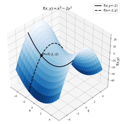
Suppose that we wish to determine the derivative of the function \(f(x)\) at \(x=-2\) and \(y=-2\). In this case, it does not make sense to simply determine the “derivative”, but rather, we must specify in which direction we want the derivative. That is, we need to specify in which direction we are interested in quantifying the rate of change of the function.
One possibility is to quantify the rate of change in the \(x\) direction. The solid line in Figure A2.2.2 shows the part of the function surface where \(y\) is fixed at -2, that is, the function evaluated as \(f(x,y=-2)\). The point \(P\) on the figure shows the value of the function when \(x=-2\) and \(y=-2\). By looking at the solid line at point \(P\), we can see that as \(x\) increases, the value of the function is gently decreasing. The derivative of \(f(x,y)\) with respect to \(x\) when \(y\) is held constant and evaluated at \(x=-2\) and \(y=-2\) is thus negative. Rather than saying “The derivative of \(f(x,y)\) with respect to \(x\) when \(y\) is held constant” we say “The partial derivative of \(f(x,y)\) with respect to \(x\)”.
Since the partial derivative is different than the ordinary derivative (as it implies that we are holding independent variables fixed), we give it a different symbol, namely, we use \(\partial\) instead of \(d\):
\[\begin{aligned}\frac{\partial f}{\partial x}=\frac{\partial}{\partial x}f(x,y)\quad\text{(Partial derivative of f with respect to x)}\end{aligned}\]
Calculating the partial derivative is very easy, as we just treat all variables as constants except for the variable with respect to which we are differentiating1. For the function \(f(x,y)=x^2-2y^2\), we have:
\[\begin{aligned} \frac{\partial f}{\partial x}&=\frac{\partial}{\partial x}(x^2-2y^2) = 2x\\[4pt] \frac{\partial f}{\partial y}&=\frac{\partial}{\partial y}(x^2-2y^2) = -4y\end{aligned}\]
At \(x=-2\), the partial derivative of \(f(x,y)\) is indeed negative, consistent with our observation that, along the solid line, at point \(P\), the function is decreasing.
A function will have as many partial derivatives as it has independent variables. Also note that, just like a normal derivative, a partial derivative is still a function. The partial derivative with respect to a variable tells us how steep the function is in the direction in which that variable increases and whether it is increasing or decreasing.
Determine the partial derivatives of \(f(x,y,z)=ax^2+byz-\sin(z)\).
Solution
In this case, we have three partial derivatives to evaluate. Note that \(a\) are \(b\) constants and can be thought of as numbers that we do not know.
\[\begin{aligned} \frac{\partial f}{\partial x}&=\frac{\partial}{\partial x}(ax^2+byz-\sin(z)) = 2ax\\[4pt] \frac{\partial f}{\partial y}&=\frac{\partial}{\partial y}(ax^2+byz-\sin(z)) = bz \\[4pt] \frac{\partial f}{\partial z}&=\frac{\partial}{\partial z}(ax^2+byz-\sin(z)) = by-\cos(z) \end{aligned}\]
Since the partial derivatives tell us how the function changes in a particular direction, we can use them to find the direction in which the function changes the most rapidly. For example, suppose that the surface from Figure A2.2.2 corresponds to a real physical surface and that we place a ball at point \(P\). We wish to know in which direction the ball will roll. The direction that it will roll in is the opposite of the direction where \(f(x,y)\) increases the most rapidly (i.e. it will roll in the direction where \(f(x,y)\) decreases the most rapidly). The direction in which the function increases the most rapidly is called the “gradient” and denoted by \(\nabla f(x,y)\).
Since the gradient is a direction, it cannot be represented by a single number. Rather, we use a “vector” to indicate this direction. Since \(f(x,y)\) has two independent variables, the gradient will be a vector with two components. The components of the gradient are given by the partial derivatives:
\[\begin{aligned} \nabla f(x,y) = \frac{\partial f}{\partial x}\hat x+\frac{\partial f}{\partial y} \hat y\end{aligned}\]
where \(\hat x\) and \(\hat y\) are the unit vectors in the \(x\) and \(y\) directions, respectively (sometimes, the unit vectors are denoted \(\hat i\) and \(\hat j\)). The direction of the gradient tells us in which direction the function increases the fastest, and the magnitude of the gradient tells us how much the function increases in that direction.
Determine the gradient of the function \(f(x,y)=x^2-2y^2\) at the point \(x=-2\) and \(y=-2\).
Solution
We have already found the partial derivatives that we need to evaluate at \(x=-2\) and \(y=-2\):
\[\begin{aligned} \frac{\partial f}{\partial x}&= 2x\\[4pt] \frac{\partial f}{\partial y}&= -4y \\[4pt] \therefore \nabla f(x,y) &= \frac{\partial f}{\partial x}\hat x+\frac{\partial f}{\partial y} \hat y \\[4pt] &=2x\hat x-4y\hat y\end{aligned}\]
Evaluating the gradient at \(x=-2\) and \(y=-2\):
\[\begin{aligned} \nabla f(x,y) &= 2x\hat x-4y\hat y\\[4pt] &=-4 \hat x + 8 \hat y\\[4pt] &=4 (-\hat x+2\hat y)\\[4pt]\end{aligned}\]
The gradient vector points in the direction \((-1,2)\). That is, the function increases the most in the direction where you would take 1 pace in the negative \(x\) direction and 2 paces in the positive \(y\) direction. You can confirm this by looking at point \(P\) in Figure A2.2.2 and imagining in which direction you would have to go to climb the surface to get the steepest climb.
The gradient is itself a function, but it is not a real function (in the sense of a real number), since it evaluates to a vector. It is a mapping from real numbers \(x,y\) to a vector. As you take more advanced calculus courses, you will eventually encounter “vector calculus”, which is just the calculus for functions of multiple variables to which you were just introduced. The key point to remember here is that the gradient can be used to find the vector that points in the direction of maximal increase of the corresponding multi-variate function. This is precisely the quantity that we need in physics to determine in which direction a ball will roll when placed on a surface (it will roll in the direction opposite to the gradient vector).
The gradient of a function of one variable, \(f(x)\), is
- undefined
- zero
- equal to its derivative
- infinite
- Answer
-
Common uses of derivatives in physics
The simplest case of using a derivative is to describe the speed of an object. If an object covers a distance \(\Delta x\) in a period of time \(\Delta t\), it’s “average speed”, \(v_{avg}\), is defined as the distance covered by the object divided by the amount of time it took to cover that distance:
\[\begin{aligned} v_{avg} = \frac{\Delta x}{\Delta t}\end{aligned}\]
If the object changes speed (for example it is slowing down) over the distance \(\Delta x\), we can still define its “instantaneous speed”, \(v\), by measuring the amount of time, \(\Delta t\), that it takes the object to cover a very small distance, \(\Delta x\). The instantaneous speed is defined in the limit where \(\Delta x \to 0\):
\[\begin{aligned} v = \lim_{\Delta x\to 0}\frac{\Delta x}{\Delta t}=\frac{dx}{dt}\end{aligned}\]
which is precisely the derivative of \(x(t)\) with respect to \(t\). \(x(t)\) is a function that gives the position, \(x\), of the object along some \(x\) axis as a function of time. The speed of the object is thus the rate of change of its position.
Similarly, if the speed is changing with time, then we can define the “acceleration”, \(a\), of an object as the rate of change of its speed:
\[\begin{aligned} a = \frac{dv}{dt}\end{aligned}\]
Footnotes
1. To take the derivative is to “differentiate”!