21.3: The magnetic force on a current-carrying wire .

review topics

Section 19.2 on the microscopic model of current.

In this section, we examine the force that is exerted by a magnetic field on a wire that carries electric current. Since a current is formed by moving charges, it is natural to expect that a wire that carries current will experience a force if immersed in a magnetic field.

Consider a vertical wire with cross-sectional area, \(A\), carrying current, \(I\), upwards that is immersed in a uniform magnetic field, \(\vec B\), into the page, as illustrated in Figure \(\PageIndex{1}\). Inside the wire, on average, electrons have a drift velocity, \(\vec v_d\), in the downwards direction (since they move in the direction opposite to that of conventional current).

Figure \(\PageIndex{1}\): A section of wire carries conventional current, \(I\), upwards while being immersed in a uniform magnetic field, \(\vec B\), into the page. We introduce the vector, \(\vec l\), to represent a section of wire of length \(l\) carrying current in the direction of \(\vec l\).

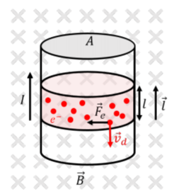
A single electron (with charge \(q=-e\)) will experience a magnetic force, \(\vec F_e\), given by:

\[\begin{aligned} \vec F_e = -e \vec v_d \times \vec B\end{aligned}\]

as illustrated in Figure \(\PageIndex{1}\). A section of wire of length, \(l\), will contain \(N=nAl\) drifting electrons, where \(n\) is the density of free electrons for the wire (the number of electrons per unit volume that are available to produce a current). Thus, the magnetic force on that section of wire will be \(N\) times the force on a single electron:

\[\begin{aligned} \vec F = N\vec F_e = nAl (-e \vec v_d \times \vec B)=-nAle \vec v_d \times \vec B\end{aligned}\]

Recall the microscopic model of current to relate the drift velocity to the conventional current in the wire:

\[\begin{aligned} I &= -nAev_d\end{aligned}\]

where the minus sign indicates that negative electrons flow in the opposite direction from the conventional current. We also introduce a vector, \(\vec l\), with a magnitude equal to the length of the section of wire, and a direction that is parallel to the conventional current (thus anti-parallel to the electron drift velocity). The force on the section of the length, \(l\), of the wire is thus given by:

\[\begin{aligned}\vec F=-nAle\vec v_{d}\times \vec B \end{aligned}\]

\[\vec F=I\vec l\times \vec B\]

Exercise \(\PageIndex{1}\)

Figure \(\PageIndex{2}\): A current carrying wire moving through a magnetic field.

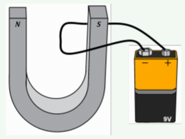
In which direction does the magnetic force point on the current-carrying wire that is placed in the magnetic field between the poles of the horseshoe magnet shown in Figure \(\PageIndex{2}\)?

1. Up.
2. Down.
3. Into the page.
4. Out of the page.

Answer

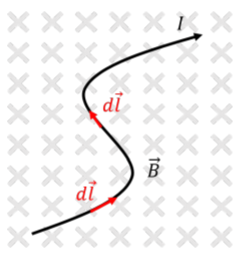
Note that if the wire is not straight, then we can model the wire as being made of many infinitesimally short sections (Figure \(\PageIndex{3}\)), of length \(dl\), and sum the forces on those sections to get the total force on a section of length, \(L\):

\[\begin{aligned} \vec F = \int_0^L I d\vec l \times \vec B\end{aligned}\]

Figure \(\PageIndex{3}\) The magnetic force on a curved current-carrying wire is obtained by modeling the forces exerted on infinitesimal sections of wire, each with length \(d\vec l\), and summing together those forces to get the total force on the wire.

Example \(\PageIndex{1}\)

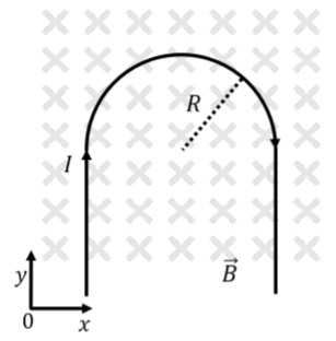
A wire carrying current, \(I\), is bent so as to have a semi-circular section with radius, \(R\), as shown in Figure \(\PageIndex{4}\). The wire is immersed in a uniform magnetic field, \(\vec B\), that is perpendicular to the plane of the wire, as shown. Using the given coordinate system, what is the net force on the wire?

Figure \(\PageIndex{4}\): A current-carrying wire with a semi-circular section is immersed in a uniform magnetic field.

Solution

We can model the wire as being made of three sections: a straight section carrying current in the positive \(y\) direction, a curved section, and another straight section carrying current in the negative \(y\) direction.

Consider the first straight section, carrying current in the positive \(y\) direction. The force on that section of wire, by the right hand rule, will be towards the left (negative \(x\) direction):

\[\begin{aligned} F_S &= I \vec l \times \vec B\\[4pt] &= I (l\hat y) \times (-B\hat z)\\[4pt] &= -IlB (\hat y \times \hat z)=-IlB\hat x\end{aligned}\]

where, \(l\), is the (unknown) length of that section of wire. The force exerted on the other straight section of wire will have the same magnitude, but the opposite direction (since the current, and thus the vector \(\vec l\), is in the opposite direction). Thus, the forces from the two straight sections of the wire cancel, as illustrated in Figure \(\PageIndex{5}\).

Figure \(\PageIndex{5}\): The magnetic force on different sections of wire.

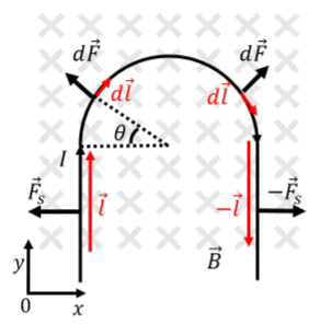
In order to calculate the force exerted on the semi-circular section, we need to add together the forces exerted on the infinitesimal sections of the wire that make up that section. Consider the magnetic force on the two infinitesimal sections illustrated in Figure \(\PageIndex{5}\). The \(x\) components of the forces will cancel, whereas the \(y\) components will add. Thus, by symmetry, we anticipate that the net force on the semi-circular section will be in the positive \(y\) direction.

Consider the small force on the section of wire located at an angle, \(\theta\), as illustrated in Figure \(\PageIndex{5}\). We can write the vector \(d\vec l\) as:

\[\begin{aligned} d\vec l = dl(\sin\theta\hat x + \cos\theta \hat y)\end{aligned}\]

Thus, the infinitesimal force on that section of wire is given by:

\[\begin{aligned} d\vec F &= I d\vec l \times \vec B = I dl(\sin\theta\hat x + \cos\theta \hat y)\times (-B\hat z)\\[4pt] &=-IBdl (\sin\theta\hat x \times \hat z + \cos\theta \hat y \times \hat z)\\[4pt] &=-IBdl (-\sin\theta \hat y + \cos\theta\hat x) \\[4pt] &= IBdl\sin\theta \hat y - IBdL\cos\theta \hat x = dF_y\hat y + dF_x \hat x\end{aligned}\]

where, in the last line, we explicitly wrote out the \(x\) and \(y\) component of the infinitesimal force vector. In order to sum together these infinitesimal forces, it is most convenient to use the angle \(\theta\) to identify each segment. \(d\theta\) is related to \(dl\), since \(dl\) is the length of the circle subtended by the infinitesimal angle \(d\theta\):

\[\begin{aligned} dl = Rd\theta\end{aligned}\]

Summing together all of the \(y\) components of the infinitesimal forces:

\[\begin{aligned} F_y = \int dF_y = \int_0^\pi IBR\sin\theta d\theta=IBR \int_0^\pi\sin\theta d\theta=2IBR\end{aligned}\]

Note that the \(x\) components sum to zero, as we predicted from symmetry:

\[\begin{aligned} F_x = \int dF_x = -\int_0^\pi IBR\cos\theta d\theta=-IBR \int_0^\pi\cos\theta d\theta=0\end{aligned}\]

The net force on the wire is thus given by:

\[\begin{aligned} \vec F = 2IBR\hat y\end{aligned}\]

Discussion

In this example we found the magnetic force on a curved section of current-carrying wire. The calculation was simplified by symmetry arguments, as we could use the right hand rule to anticipate that the force would have no component in the \(x\) direction. This is because there is as much current flowing in the positive \(y\) direction as there is in the negative \(y\) direction, so that the corresponding forces cancel. There is however a net flow of charges in the positive \(x\) direction, leading to a net force in the positive \(y\) direction. As a corollary, the net magnetic force on any closed loop of current must be zero.