1.2: Position, Displacement, Velocity

Kinematics is the part of mechanics that deals with the mathematical description of motion, leaving aside the question of what causes an object to move in a certain way. Kinematics, therefore, does not include such things as forces or energy, which fall instead under the heading of dynamics. It may be said, then, that kinematics by itself is not true physics, but only applied mathematics; yet it is still an essential part of classical mechanics, and its most natural starting point. This chapter (and parts of the next one) will introduce the basic concepts and methods of kinematics in one dimension.

Position

As stated in the previous section, we are initially interested only in describing the motion of a “particle,” which can be thought of as a mathematical point in space. (Later on we will see that, even for an extended object or system, it is often useful to consider the motion of a specific point that we call the system’s center of mass.) A point in three dimensions can be located by giving three numbers, known as its Cartesian coordinates (or, more simply, its coordinates). In two dimensions, this works as shown in Figure \(\PageIndex{1}\) below. As you can see, the coordinates of a point just tell us how to find it by first moving a certain distance \(x\), from a previously-agreed origin, along a horizontal (or \(x\)) axis, and then a certain distance \(y\) along a vertical (or \(y\)) axis. (Or, of course, you could equally well first move vertically and then horizontally.)

Figure \(\PageIndex{1}\): The position vector, \( \vec r\), of a point, and its \(x\) and \(y\) components (the point's coordinates).

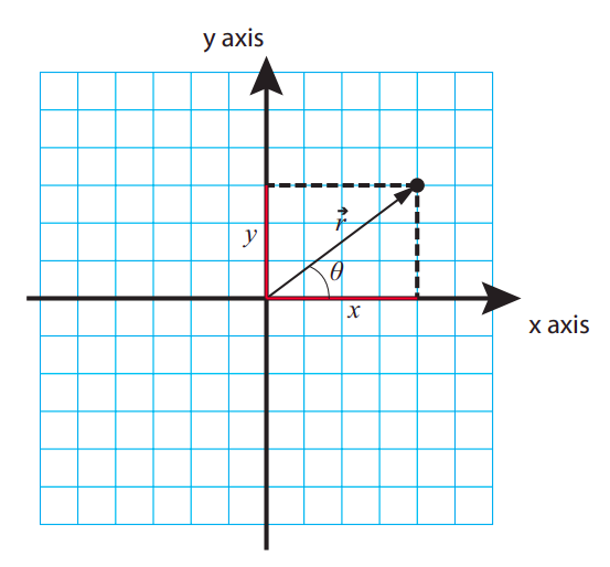
The quantities \(x\) and \(y\) are taken to be positive or negative depending on what side of the origin the point is on. Typically, we will always start by choosing a positive direction for each axis, as the direction along which the algebraic value of the corresponding coordinate increases. This is often chosen to be to the right for the horizontal axis, and upwards for the vertical axis, but there is nothing that says we cannot choose a different convention if it turns out to be more convenient. In Figure \(\PageIndex{1}\), the arrows on the axes denote the positive direction for each. Going by the grid, the coordinates of the point shown are \(x\) = 4 units, \(y\) = 3 units.

In two or three dimensions (and even, in a sense, in one dimension), the coordinates of a point can be interpreted as the components of a vector that we call the point’s position vector, and denote by \(\vec r\) (sometimes boldface letters are used for vectors, instead of an arrow on top; in that case, the position vector would be denoted by r). A vector is a mathematical object, with specific geometric and algebraic properties, that physicists use to represent a quantity that has both a magnitude and a direction. The magnitude of the position vector in Figure \(\PageIndex{1}\) is just the length of the arrow, which is to say, 5 length units (by the Pythagorean theorem, the length of \(\vec r\), which we will often write using absolute value bars as \(|\vec{r}|\), is equal to \( \sqrt{x^{2}+y^{2}} \)); this is just the straight-line distance of the point to the origin. The direction of \(\vec r\), on the other hand, can be specified in a number of ways; a common convention is to give the value of the angle that it makes with the positive \(x\) axis, which I have denoted in the figure as \(\theta\) (in this case, you can verify that \( \theta=\tan ^{-1}(y / x)=36.9^{\circ} \)). In three dimensions, two angles would be needed to completely specify the direction of \(\vec r\).

As you can see, giving the magnitude and direction of \(\vec r\) is a way to locate the point that is completely equivalent to giving its coordinates \(x\) and \(y\). By the same token, the coordinates \(x\) and \(y\) are a way to specify the vector \(\vec r\) that is completely equivalent to giving its magnitude and direction. As I stated above, we call x and y the components (or sometimes, to be more specific, the Cartesian components) of the vector \(\vec r\). In a sense all the vectors that will be introduced later on this semester will derive their geometric and algebraic properties from the position vector \(\vec r\), so once you know how to deal with one vector, you can deal with them all. The geometric properties (by which I mean, how to relate a vector’s components to its magnitude and direction) I have just covered, and will come back to later on in this chapter, and again in Chapter 8; the algebraic properties (how to add vectors and multiply them by ordinary numbers, which are called scalars in this context) I will introduce along the way.

For the first few chapters this semester, we are going to be primarily concerned with motion in one dimension (that is to say, along a straight line, backwards or forwards), in which case all we need to locate a point is one number, its \(x\) (or \(y\), or \(z\)) coordinate; we do not then need to worry particularly about vector algebra. Alternatively, we can simply say that a vector in one dimension is essentially the same as its only component, which is just a positive or negative number (the magnitude of the number being the magnitude of the vector, and its sign indicating its direction), and has the algebraic properties that follow naturally from that.

The description of the motion that we are aiming for is to find a function of time, which we denote by \(x(t)\), that gives us the point’s position (that is to say, the value of \(x\)) for any value of the time parameter, \(t\). (See Equation (\ref{eq:10}), below, for an example.) Remember that \(x\) stands for a number that can be positive or negative (depending on the side of the origin the point is on), and has dimensions of length, so when giving a numerical value for it you must always include the appropriate units (meters, centimeters, miles...). Similarly, \(t\) stands for the time elapsed since some more or less arbitrary “origin of time,” or time zero. Normally \(t\) should always be positive, but in special cases it may make sense to consider negative times (think of how we count years: “AD” would correspond to “positive” and “BC” would correspond to negative—the difference being that there is actually no year zero!). Anyway, \(t\) also is a number with dimensions, and must be reported with its appropriate units: seconds, minutes, hours, etc.

Figure \(\PageIndex{2}\): A possible position vs. time graph for an object moving in one dimension

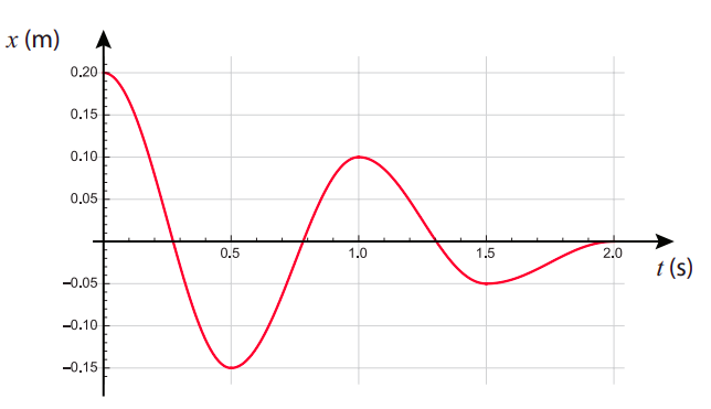
We will be often interested in plotting the position of an object as a function of time—that is to say, the graph of the function \(x(t)\). This may, in principle, have any shape, as you can see in Figure \(\PageIndex{2}\) above. In the lab, you will have a chance to use a position sensor that will automatically generate graphs like that for you on the computer, for any moving object that you aim the position sensor at. It is, therefore, important that you learn how to “read” such graphs. For example, Figure \(\PageIndex{2}\) shows an object that starts, at the time \(t\) = 0, a distance 0.2 m away and to the right of the origin (so \(x(0)\) = 0.2 m), then moves in the negative direction to \(x\) = −0.15 m, which it reaches at \(t\) = 0.5 s; then turns back and moves in the opposite direction until it reaches the point \(x\) = 0.1 m, turns again, and so on. Physically, this could be tracking the damped oscillations of a system such as an object attached to a spring and sliding over a surface that exerts a friction force on it (see Example 11.5.1).

Displacement

In one dimension, the displacement of an object over a given time interval is a quantity that we denote as \(\Delta x\), and equals the difference between the object’s initial and final positions (in one dimension, we will often call the “position coordinate” simply the “position,” for short):

\[ \Delta x=x_{f}-x_{i} \label{eq:1} \]

Here the subscript \(i\) denotes the object’s position at the beginning of the time interval considered, and the subscript \(f\) its position at the end of the interval. The symbol \(\Delta\) will consistently be used throughout this book to denote a change in the quantity following the symbol, meaning the difference between its initial value and its final value. The time interval itself will be written as ∆t and can be expressed as

\[ \Delta t=t_{f}-t_{i} \]

where again \(t_i\) and \(t_f\) are the initial and final values of the time parameter (imagine, for instance, that you are reading time in seconds on a digital clock, and you are interested in the change in the object’s position between second 130 and second 132: then \(t_i\) = 130 s, \(t_2\) = 132 s, and \(\Delta t\) = 2 s).

You can practice reading off displacements from Figure \(\PageIndex{2}\). The displacement between \(t_i\) = 0.5 s and \(t_f\) = 1 s, for instance, is 0.25 m ( \(x_i\) = −0.15 m, \(x_f\) = 0.1 m). On the other hand, between \(t_i\) = 1 s and \(t_f\) = 1.3 s, the displacement is \(\Delta x\) = 0 − 0.1 = −0.1 m

Notice two important things about the displacement. First, it can be positive or negative. Positive means the object moved, overall, in the positive direction; negative means it moved, overall, in the negative direction. Second, even when it is positive, the displacement does not always equal the distance traveled by the object (distance, of course, is always defined as a positive quantity), because if the object “doubles back” on its tracks for some distance, that distance does not count towards the overall displacement. For instance, looking again at Figure \(\PageIndex{2}\), in between the times \(t_i\) = 0.5 s and \(t_f\) = 1.5 s the object moved first 0.25 m in the positive direction, and then 0.15 m in the negative direction, for a total distance traveled of 0.4 m; however, the total displacement was just 0.1 m.

In spite of these quirks, the total displacement is, mathematically, a useful quantity, because often we will have a way (that is to say, an equation) to calculate \(\Delta x\) for a given interval, and then we can rewrite Equation (\ref{eq:1}) so that it reads

\[ x_{f}=x_{i}+\Delta x .\]

That is to say, if we know where the object started, and we have a way to calculate \(\Delta x\), we can easily figure out where it ended up. You will see examples of this sort of calculation in the homework later on.

Extension to Two Dimensions

In two dimensions, we write the displacement as the vector

\[ \Delta \vec{r}=\vec{r}_{f}-\vec{r}_{i} .\]

The components of this vector are just the differences in the position coordinates of the two points involved; that is, \( (\Delta \vec r)_x \) (a subscript \(x\), \(y\), etc., is a standard way to represent the \(x\), \(y\) . . . component of a vector) is equal to \(x_f - x_i\), and similarly \((\Delta \vec{r})_{y}=y_{f}-y_{i}\).

Figure \(\PageIndex{3}\): The displacement vector for a particle that was initially at a point with position vector \(\vec r_i\) and ended up at a point with position vector \(\vec r_f\) is the difference of the position vectors.

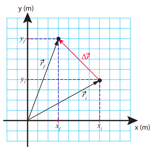
Figure \(\PageIndex{3}\) shows how this makes sense. The \(x\) component of \(\Delta \vec r\) in the figure is \(\Delta x\) = 3 − 7 = −4 m; the \(y\) component is \(\Delta y\) = 8 − 4 = 4 m. This basically shows you how to subtract (and, by extension, add, since \( \vec{r}_{f}=\vec{r}_{i}+\Delta \vec{r}\) ) vectors: you just subtract (or add) the corresponding components. Note how, by the Pythagorean theorem, the length (or magnitude) of the displacement vector, \( |\Delta \vec{r}| = \sqrt{\left(x_{f}-x_{i}\right)^{2}+\left(y_{f}-y_{i}\right)^{2}} \), equals the straight-line distance between the initial point and the final point, just as in one dimension; of course, the particle could have actually followed a very different path from the initial to the final point, and therefore traveled a different distance.

Velocity

Average Velocity

If you drive from Fayetteville to Fort Smith in 50 minutes, your average speed for the trip is calculated by dividing the distance of 59.2 mi by the time interval:

\[ \text { average speed }=\frac{\text { distance }}{\Delta t}=\frac{59.2 \: \mathrm{mi}}{50 \: \mathrm{min}}=\frac{59.2 \: \mathrm{mi}}{50 \: \mathrm{min}} \times \frac{60 \: \mathrm{min}}{1 \: \mathrm{hr}}=71.0 \: \mathrm{mph} \label{eq:5} \]

(this equation, incidentally, also shows you how to convert units, and how you will be expected to work with significant figures this semester: the rule of thumb is, keep four significant figures in all intermediate calculations, and report three in the final result).

The way we define average velocity is similar to average speed, but with one important difference: we use the displacement, instead of the distance. So, the average velocity \(v_{av}\) of an object, moving along a straight line, over a time interval \(\Delta t\) is

\[ v_{a v}=\frac{\Delta x}{\Delta t} \label{eq:6} .\]

This definition has all the advantages and the quirks of the displacement itself. On the one hand, it automatically comes with a sign (the same sign as the displacement, since \(\Delta t\) will always be positive), which tells us in what direction we have been traveling. On the other hand, it may not be an accurate estimate of our average speed, if we doubled back at all. In the most extreme case, for a roundtrip (leave Fayetteville and return to Fayetteville), the average velocity would be zero, since \(x_f = x_i\) and therefore \(\Delta x\) = 0.

It is clear that this concept is not going to be very useful in general, if the object we are tracking has a chance to double back in the time interval \(\Delta t\). A way to prevent this from happening, and also getting a more meaningful estimate of the object’s speed at any instant, is to make the time interval very small. This leads to a new concept, that of instantaneous velocity.

Instantaneous Velocity

We define the instantaneous velocity of an object (a “particle”), at the time \(t = t_i\), as the mathematical limit

\[ v=\lim _{\Delta t \rightarrow 0} \frac{\Delta x}{\Delta t} \label{eq:7} .\]

The meaning of this is the following. Suppose we compute the ratio \(\Delta x/\Delta t\) over successively smaller time intervals \(\Delta t\) (all of them starting at the same time \(t_i\)). For instance, we can start by making \(t_f = t_i + 1\: s\), then try \(t_f = t_i + 0.5 \: s\), then \(t_f = t_i + 0.1 \: s\), and so on. Naturally, as the time interval becomes smaller, the corresponding displacement will also become smaller—the particle has less and less time to move away from its initial position, \(x_i\). The hope is that the successive ratios \(\Delta x/\Delta t\) will converge to a definite value: that is to say, that at some point we will start getting very similar values, and that beyond a certain point making \(\Delta t\) any smaller will not change any of the significant digits of the result that we care about. This limit value is the instantaneous velocity of the object at the time \(t_i\).

When you think about it, there is something almost a bit self-contradictory about the concept of instantaneous velocity. You cannot (in practice) determine the velocity of an object if all you are given is a literal instant. You cannot even tell if the object is moving, if all you have is one instant! Motion requires more than one instant, the passage of time. In fact, all the “instantaneous” velocities that we can measure, with any instrument, are always really average velocities, only the average is taken over very short time intervals. Nevertheless, the fact is that for any reasonably well-behaved position function \(x(t)\), the limit in Equation (\ref{eq:7}) is mathematically well-defined, and it equals what we call, in calculus, the derivative of the function \(x(t)\):

\[ v=\lim _{\Delta t \rightarrow 0} \frac{\Delta x}{\Delta t}=\frac{d x}{d t} \label{eq:8} .\]

Figure \(\PageIndex{4}\): The slope of the green segment is the average velocity for the time interval \(\Delta t\) shown. As \(\Delta t\) becomes smaller, this approaches the slope of the tangent at the point \((t_i, x_i)\)

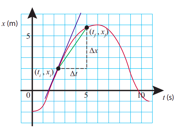
In fact, there is a nice geometric interpretation for this quantity: namely, it is the slope of a line tangent to the \(x\)-vs-\(t\) curve at the point , \((t_i, x_i)\). As Figure \(\PageIndex{4}\) shows, the average velocity \(\Delta x/\Delta t\) is the slope (rise over run) of a line segment drawn from the point \((t_i, x_i)\) to the point \((t_f, x_f)\) (the green line in the figure). As we make the time interval smaller, by bringing \(t_f\) closer to \(t_i\) (and hence, also, \(x_f\) closer to \(x_i\)), the slope of this segment will approach the slope of the tangent line at \((t_i, x_i)\) (the blue line), and this will be, by the definition (\ref{eq:7}), the instantaneous velocity at that point.

This geometric interpretation makes it easy to get a qualitative feeling, from the position-vs-time graph, for when the particle is moving more or less fast. A large slope means a steep rise or fall, and that is when the velocity will be largest—in magnitude. A steep rise means a large positive velocity, whereas a steep drop means a large negative velocity, by which I mean a velocity that is given by a negative number which is large in absolute value. In the future, to simplify sentences like this one, I will just use the word “speed” to refer to the magnitude (that is to say, the absolute value) of the instantaneous velocity. Thus, speed (like distance) is always a positive number, by definition, whereas velocity can be positive or negative; and a steep slope (positive or negative) means the speed is large there.

Conversely, looking at the sample \(x\)-vs-\(t\) graphs in this chapter, you may notice that there are times when the tangent is horizontal, meaning it has zero slope, and so the instantaneous velocity at those times is zero (for instance, at the time \(t\) = 1.0 s in Figure \(\PageIndex{2}\)). This makes sense when you think of what the particle is actually doing at those special times: it is just changing direction, so its velocity is going, for instance, from positive to negative. The way this happens is, it slows down, down... the velocity gets smaller and smaller, and then, for just an instant (literally, a mathematical point in time), it becomes zero before, the next instant, going negative.

We will be coming back to this “reading of graphs” in the lab and the homework, as well as in the next chapter, when we introduce the concept of acceleration.

Motion With Constant Velocity

If the instantaneous velocity of an object never changes, it means that it is always moving in the same direction with the same speed. In that case, the instantaneous velocity and the average velocity coincide, and that means we can write \(v = \Delta x/ \Delta t\) (where the size of the interval \(\Delta t\) could now be anything), and rewrite this equation in the form

\[ \Delta x = v \Delta t \label{eq:9} \]

which is the same as

\[ x_{f}-x_{i}=v\left(t_{f}-t_{i}\right) \nonumber \]

Now suppose we keep \(t_i\) constant (that is, we fix the initial instant) but allow the time \(t_f\) to change, so we will just write \(t\) for an arbitrary value of \(t_f\) , and \(x\) for the corresponding value of \(x_f\) . We end up with the equation

\[ x-x_{i}=v\left(t-t_{i}\right) \nonumber \]

which we can also write as

\[ x(t)=x_{i}+v\left(t-t_{i}\right) \label{eq:10}\]

after some rearranging, and where the notation \(x(t)\) has been introduced to emphasize that we want to think of \(x\) as a function of \(t\). This is, not surprisingly, the equation of a straight line—a “curve” which is its own tangent and always has the same slope.

(Please make sure that you are not confused by the notation in Equation (\ref{eq:10}). The parentheses around the \(t\) on the left-hand side mean that we are considering the position \(x\) as a function of \(t\). On the other hand, the parentheses around the quantity \(t − t_i\) on the right-hand side mean that we are multiplying this quantity by \(v\), which is a constant here. This distinction will be particularly important when we introduce the function \(v(t)\) next.)

Either one of equations (\ref{eq:9}) or (\ref{eq:11}) can be used to solve problems involving motion with constant velocity, and again you will see examples of this in the homework.

Motion With Changing Velocity

If the velocity changes with time, obtaining an expression for the position of the object as a function of time may be a nontrivial task. In the next chapter we will study an important special case, namely, when the velocity changes at a constant rate (constant acceleration).

For the most general case, a graphical method that is sometimes useful is the following. Suppose that we know the function \(v(t)\), and we graph it, as in Figure \(\PageIndex{5}\) below. Then the area under the curve in between any two instants, say \(t_i\) and \(t_f\) , is equal to the total displacement of the object over that time interval.

The idea involved is known in calculus as integration, and it goes as follows. Suppose that I break

Figure \(\PageIndex{5}\): How to get the displacement from the area under the \(v\)-vs-\(t\) curve.

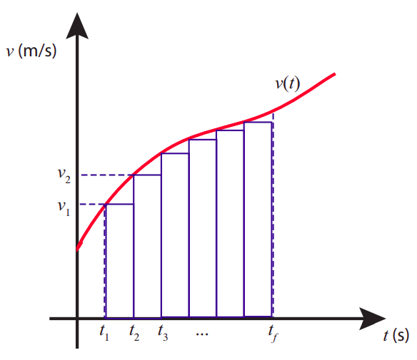
down the interval from \(t_i\) to \(t_f\) into equally spaced subintervals, beginning at the time \(t_i\) (which I am, equivalently, going to call \(t_1\), that is, \(t_{1} \equiv t_{i}\), so I have now \(t_1\), \(t_2\), \(t_3\),...\(t_f\) ). Now suppose I treat the object’s motion over each subinterval as if it were motion with constant velocity, the velocity being that at the beginning of the subinterval. This, of course, is only an approximation, since the velocity is constantly changing; but, if you look at Figure \(\PageIndex{5}\), you can convince yourself that it will become a better and better approximation as I increase the number of intermediate points and the rectangles shown in the figure become narrower and narrower. In this approximation, the displacement during the first subinterval would be

\[ \Delta x_{1}=v_{1}\left(t_{2}-t_{1}\right) \label{eq:11} \]

where \(v_1 = v(t_1)\); similarly, \(\Delta x_2 = v_2(t_3 − t_2)\), and so on.

However, Equation (\ref{eq:11}) is just the area of the first rectangle shown under the curve in Figure \(\PageIndex{5}\) (the base of the rectangle has “length” \(t_2 − t_1\), and its height is \(v_1\)). Similarly for the second rectangle, and so on. So the sum \(\Delta x_1+\Delta x_2+...\) is both an approximation to the area under the \(v\)-vs-\(t\) curve, and an approximation to the total displacement \(\Delta t\). As the subdivision becomes finer and finer, and the rectangles narrower and narrower (and more numerous), both approximations become more and more accurate. In the limit of “infinitely many,” infinitely narrow rectangles, you get both the total displacement and the area under the curve exactly, and they are both equal to each other. Mathematically, we would write

\[ \Delta x=\int_{t_{i}}^{t_{f}} v(t) d t \label{eq:12} \]

where the stylized “S” (for “sum”) on the right-hand side is the symbol of the operation known as integration in calculus. This is essentially the inverse of the process know as differentiation, by which we got the velocity function from the position function, back in Equation (\ref{eq:8}).

This graphical method to obtain the displacement from the velocity function is sometimes useful, if you can estimate the area under the \(v\)-vs-\(t\) graph reliably. An important point to keep in mind is that rectangles under the horizontal axis (corresponding to negative velocities) have to be added as having negative area (since the corresponding displacement is negative); see example 1.5.1 at the end of this chapter.

Extension to Two Dimensions

In two (or more) dimensions, you define the average velocity vector as a vector \(\vec v_{av}\) whose components are \(v_{av,x} = \Delta x/ \Delta t\), \(v_{av,y} = \Delta y/ \Delta t\), and so on (where \(\Delta x\), \(\Delta y\),... are the corresponding components of the displacement vector \(\Delta \vec r \)). This can be written equivalently as the single vector equation

\[ \vec{v}_{a v}=\frac{\Delta \vec{r}}{\Delta t} \label{eq:13} .\]

This tells you how to multiply (or divide) a vector by an ordinary number: you just multiply (or divide) each component by that number. Note that, if the number in question is positive, this operation does not change the direction of the vector at all, it just scales it up or down (which is why ordinary numbers, in this context, are called scalars). If the scalar is negative, the vector’s direction is flipped as a result of the multiplication. Since \(\Delta t\) in the definition of velocity is always positive, it follows that the average velocity vector always points in the same direction as the displacement, which makes sense.

To get the instantaneous velocity, you just take the limit of the expression (\ref{eq:13}) as \(\Delta t \rightarrow 0\), for each component separately. The resulting vector \(\vec v\) has components \(v_x = \lim_{\Delta t \rightarrow 0} \frac{\Delta x}{\Delta t} \), etc., which can also be written as \(v_x = dx/dt, v_y = dy/dt\), . . ..

All the results derived above hold for each spatial dimension and its corresponding velocity component. For instance, the graphical method shown in Figure \(\PageIndex{5}\) can always be used to get \(\Delta x\) if the function \(v_x(t)\) is known, or equivalently to get \(\Delta y\) if you know \(v_y(t)\), and so on.

Introducing the velocity vector at this point does cause a little bit of a notational difficulty. For quantities like \(x\) and \(\Delta x\), it is pretty obvious that they are the \(x\) components of the vectors \(\vec r\) and \(\Delta \vec r\) respectively; however, the quantity that we have so far been calling simply \(v\) should more properly be denoted as \(v_x\) (or \(v_y\) if the motion is along the \(y\) axis). In fact, there is a convention that if you use the symbol for a vector without the arrow on top or any \(x\), \(y\), . . . subscripts, you must mean the magnitude of the vector. In this book, however, I have decided not to follow that convention, at least not until we get to Chapter 8 (and even then I will use it only for forces). This is because we will spend most of our time dealing with motion in only one dimension, and it makes the notation unnecessarily cumbersome to keep having to write the \(x\) or \(y\) subscripts on every component of every vector, when you really only have one dimension to worry about in the first place. So \(v\) will, throughout, refer to the relevant component of the velocity vector, to be inferred from the context, until we get to Chapter 8 and actually need to deal with both a \(v_x\) and a \(v_y\) explicitly.

Finally, notice that the magnitude of the velocity vector, \(|\vec{v}|=\sqrt{v_{x}^{2}+v_{y}^{2}+v_{z}^{2}}\), is equal to the instantaneous speed, since, as \(\Delta t \rightarrow 0\), the magnitude of the displacement vector, \(|\Delta vec r |\), becomes the actual distance traveled by the object in the time interval \(\Delta t\).