
13.2: Introducing Temperature
- Page ID
- 22282

Temperature and Heat Capacity
The change in perspective that I just mentioned also means that it is not easy to even define temperature, beyond our natural intuition of “hot” and “cold,” or the somewhat circular notion that temperature is simply “what thermometers measure.” Roughly speaking, though, temperature is a measure of the amount (or, to be somewhat more precise, the concentration) of thermal energy in an object. When we directly put an amount of thermal energy, \(\Delta E_{th}\) (what we will be calling heat in a moment), in an object, we typically observe its temperature to increase in a way that is approximately proportional to \(\Delta E_{th}\), at least as long as \(\Delta E_{th}\) is not too large:
\[ \Delta T=\frac{\Delta E_{t h}}{C} \label{eq:13.1} .\]
The proportionality constant \(C\) is called the heat capacity of the object: according to Equation (\ref{eq:13.1}), a system with a large heat capacity could absorb (or give off—the equation is supposed to apply in either case) a large amount of thermal energy without experiencing a large change in temperature. If the system does not do any work in the process (recall Equation (7.4.8)!), then its internal energy will increase (or decrease) by exactly the same amount of thermal energy it has taken in (or given off)1, and we can use the heat capacity2 to, ultimately, relate the system’s temperature to its energy content in a one-to-one-way.
What is found experimentally is that the heat capacity of a homogeneous object (that is, one made of just one substance) is, in general, proportional to its mass. This is why, instead of tables of heat capacities, what we compile are tables of specific heats, which are heat capacities per kilogram (or sometimes per mole, or per cubic centimeter... but all these things are ultimately proportional to the object’s mass). In terms of a specific heat \(c = C/m\), and again assuming no work done or by the system, we can rewrite Equation (\ref{eq:13.1}) to read
\[ \Delta E_{s y s}=m c \Delta T \label{eq:13.2} \]
or, again,
\[ \Delta T=\frac{\Delta E_{s y s}}{m c} \label{eq:13.3} \]
which shows what I said above, that temperature really measures, not the total energy content of an object, but its concentration—the thermal energy “per unit mass,” or, if you prefer (and somewhat more fundamentally) “per molecule.” An object can have a great deal of thermal energy just by virtue of being huge, and yet still be pretty cold (water in the ocean is a good example).
In fact, we can also rewrite Eqs. (\ref{eq:13.1}–\ref{eq:13.3}) in the (somewhat contrived-looking) form
\[ C=m c=m \frac{\Delta E_{s y s} / m}{\Delta T} \label{eq:13.4} \]
which tells you that an object can have a large heat capacity in two ways: one is simply to have a lot of mass, and the other is to have a large specific heat. The first of these ways is kind of boring (but potentially useful, as I will discuss below); the second is interesting, because it means that a relatively large change in the internal energy per molecule (roughly speaking, the numerator of (\ref{eq:13.4})) will only show as a relatively small change in temperature (the denominator of (\ref{eq:13.4}); a large numerator and a small denominator make for a large fraction!).
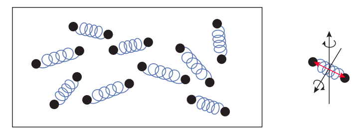
Put differently, and somewhat fancifully, substances with a large specific heat are very good at hiding their thermal energy from thermometers (see Figure \(\PageIndex{1}\) for an example). This, as I said, is an interesting observation, but it also means that measuring heat capacities—or, for that matter, measuring temperature itself—may not be an easy matter. How do we get at the object’s internal energy if not through its temperature? Where does one start?
1If the system does do some work (or has work done on it), then Equation (13.3.1) applies.
2Which, it must be noted, may also be a function of the system’s temperature—another complication we will cheerfully ignore here.
The Gas Thermometer
A good start, at least conceptually, is provided by looking at a system that has no place to hide its thermal energy—it has to show it all, have it, as it were, in full view all the time. Such a system is what has come to be known as an ideal gas—which we model, microscopically, as a collection of molecules (or, more properly, atoms) with no dimension and no structure: just pointlike things whizzing about and continually banging into each other and against the walls of their container. For such a system the only possible kind of internal energy is the sum of the molecules’ translational kinetic energy. We may expect this to be easily detected by a thermometer (or any other energy-sensitive probe), because as the gas molecules bang against the thermometer, they will indirectly reveal the energy they carry, both by how often and how hard they collide.
As it turns out, we can be a lot more precise than that. We can analyze the theoretical model of an ideal gas that we have just described fairly easily, using nothing but the concepts we have introduced earlier in the semester (plus a few simple statistical ideas) and obtain the following result for the gas’ pressure and volume:
\[ P V=\frac{2}{3} N\left\langle K_{\text {trans}}\right\rangle \label{eq:13.5} \]
where \(N\) is the total number of molecules, and \(\left\langle K_{\text {trans}}\right\rangle\) is the average translational kinetic energy per molecule. Now, you are very likely to have seen, in high-school chemistry, the experimentally derived “ideal gas law,”
\[ P V=n R T \label{eq:13.6} \]
where \(n\) is the number of moles, and \(R\) the “ideal gas constant.” Comparing Equation (\ref{eq:13.5}) (a theoretical prediction for a mathematical model) and Equation (\ref{eq:13.6}) (an empirical result approximately valid for many real-world gases under a wide range of pressure and temperature, where “temperature” literally means simply “what any good thermometer would measure”) immediately tells us what temperature is, at least for this extremely simple system: it is just a measure of the average (translational) kinetic energy per molecule.
It would be tempting to leave it at that, and immediately generalize the result to all kinds of other systems. After all, presumably, a thermometer inserted in a liquid is fundamentally responding to the same thing as a thermometer inserted in an ideal gas: namely, to how often, and how hard, the liquid’s molecules bang against the thermometer’s wall. So we can assume that, in fact, it must be measuring the same thing in both cases—and that would be the average translational kinetic energy per molecule. Indeed, there is a result in classical statistical mechanics that states that for any system (liquid, solid, or gas) in “thermal equilibrium” (a state that I will define more precisely later), the average translational kinetic energy per molecule must be
\[ \left\langle K_{\text {trans}}\right\rangle=\frac{3}{2} k_{B} T \label{eq:13.7} \]
where \(k_B\) is a constant called Boltzmann’s constant (\(k_B\) = 1.38×10⁻²³ J/K), and \(T\), as in Equation (\ref{eq:13.6}) is measured in degrees Kelvin.
There is nothing wrong with this way to think about temperature, except that it is too selflimiting. To simply identify temperature with the translational kinetic energy per molecule leaves out a lot of other possible kinds of energy that a complex system might have (a sufficiently complex molecule may also rotate and vibrate, for instance, as shown in Figure \(\PageIndex{1}\); these are some of the ways the molecule can “hide” its energy from the thermometer, as I suggested above). Typically, all those other forms of internal energy also go up as the temperature increases, so it would be at least a bit misleading to think of the temperature as having to do with only \(K_{trans}\), Equation (\ref{eq:13.7}) notwithstanding. Ultimately, in fact, it is the total internal energy of the system that we want to relate to the temperature, which means having to deal with those pesky specific heats I introduced in the previous section. (As an aside, the calculation of specific heats was one of the great challenges to the theoretical physicists of the late 19th and early 20th century, and eventually led to the introduction of quantum mechanics—but that is another story!)
In any case, the ideal gas not only provides us with an insight into the microscopic picture behind the concept of temperature, it may also serve as a thermometer itself. Equation (\ref{eq:13.6}) shows that the volume of an ideal gas held at constant pressure will increase in a way that’s directly proportional to the temperature. This is just how a conventional, old-fashioned mercury thermometer worked—as the temperature rose, the volume of the liquid in the tube went up. The ideal gas thermometer is a bit more cumbersome (a relatively small temperature change may cause a pretty large change in volume), but, as I stated earlier, typically works well over a very large temperature range.
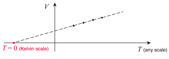
By using an ideal (or nearly ideal) gas as a thermometer, based on Equation (\ref{eq:13.6}), we are, in fact, implicitly defining a specific temperature scale, the Kelvin scale (indeed, you may recall that for Equation (\ref{eq:13.6}) to work, the temperature must be measured in degrees Kelvin). The zero point of that scale (what we call absolute zero) is the theoretical point at which an ideal gas would shrink to precisely zero volume. Of course, no gas stays ideal (or even gaseous!) at such low temperatures, but the point can easily be found by extrapolation: for instance, imagine plotting experimental values of \(V\) vs \(T\), at constant pressure, for a nearly ideal gas, using any kind of thermometer scale to measure \(T\), over a wide range of temperatures. Then, connect the points by a straight line, and extend the line to where it crosses the \(T\) axis (so \(V\) = 0); that point gives you the value of absolute zero in the scale you were using, such as −273.15 Celsius, for instance, or −459.67 Fahrenheit.
The connection between Kelvin (or absolute) temperature and microscopic motion expressed by equations like (\ref{eq:13.5}) through (\ref{eq:13.7}) immediately tells us that as you lower the temperature the atoms in your system will move more and more slowly, until, when you reach absolute zero, all microscopic motion would cease. This does not quite happen, because of quantum mechanics, and we also believe that it is impossible to really reach absolute zero for other reasons, but it is true to a very good approximation, and experimentalists have recently become very good at cooling small ensembles of atoms to temperatures extremely close to absolute zero, where the atoms move, literally, slower than snails (instead of whizzing by at close to the speed of sound, as the air molecules do at room temperature).
The Zero-th Law
Historically, thermometers became useful because they gave us a way to quantify our natural perception of cold and hot, but the quantity they measure, temperature, would have been pretty useless if it had not exhibited an important property, which we naturally take for granted, but which is, in fact, surprisingly not trivial. This property, which often goes by the name of the zero-th law of thermodynamics, can be stated as follows:
Suppose you place two systems \(A\) and \(B\) in contact, so they can directly exchange thermal energy (more about this in the next section), while isolating them from the rest of the world (so their joint thermal energy has no other place to go). Then, eventually, they will reach a state, called thermal equilibrium, in which they will both have the same temperature.
This is important for many reasons, not the least of which being that that is what allows us to measure temperature with a thermometer in the first place: the thermometer tells us the temperature of the object with which we place it in contact, by first adopting itself that temperature! Of course, a good thermometer has to be designed so that it will do that while changing the temperature of the system being measured as little as possible; that is to say, the thermometer has to have a much smaller heat capacity than the system it is measuring, so that it only needs to give or take a very small amount of thermal energy in order to match its temperature. But the main point here is that the match actually happens, and when it does, the temperature measured by the thermometer will be the same for any other systems that are, in turn, in thermal equilibrium with—that is, at the same temperature as—the first one.
The zero-th law only assures us that thermal equilibrium will eventually happen, that is, the two systems will eventually reach one and the same temperature; it does not tell us how long this may take, nor even, by itself, what that final temperature will be. The latter point, however, can be easily determined if you make use of conservation of energy (the first law, coming up!) and the concept of heat capacity introduced above (think about it for a minute).
Still, as I said above, this result is far from trivial. Just imagine, for instance, two different ideal gases, whose molecules have different masses, that you bring to a state of joint thermal equilibrium. Equations (\ref{eq:13.5}) through (\ref{eq:13.7}) tell us that in this final state the average translational kinetic energy of the “\(A\)” molecules and the “\(B\)” molecules will be the same. This means, in particular, that the more massive molecules will end up moving more slowly, on average, so \(m_av^2_{a,av} = m_bv^2_{b,av}\). But why is that? Why should it be the kinetic energies that end up matching, on average, and not, say, the momenta, or the molecular speeds themselves? The result, though undoubtedly true, defied a rigorous mathematical proof for decades, if not centuries; I am not sure that a rigorous proof exists, even now.