7.6: Linear Stark Effect

Last updated
Save as PDF

Page ID: 1221

$ \newcommand{\vecs}[1]{\overset { \scriptstyle \rightharpoonup} {\mathbf{#1}} } $ $ \newcommand{\vecd}[1]{\overset{-\!-\!\rightharpoonup}{\vphantom{a}\smash {#1}}} $$\newcommand{\id}{\mathrm{id}}$ $ \newcommand{\Span}{\mathrm{span}}$ $ \newcommand{\kernel}{\mathrm{null}\,}$ $ \newcommand{\range}{\mathrm{range}\,}$ $ \newcommand{\RealPart}{\mathrm{Re}}$ $ \newcommand{\ImaginaryPart}{\mathrm{Im}}$ $ \newcommand{\Argument}{\mathrm{Arg}}$ $ \newcommand{\norm}[1]{\| #1 \|}$ $ \newcommand{\inner}[2]{\langle #1, #2 \rangle}$ $ \newcommand{\Span}{\mathrm{span}}$ $\newcommand{\id}{\mathrm{id}}$ $ \newcommand{\Span}{\mathrm{span}}$ $ \newcommand{\kernel}{\mathrm{null}\,}$ $ \newcommand{\range}{\mathrm{range}\,}$ $ \newcommand{\RealPart}{\mathrm{Re}}$ $ \newcommand{\ImaginaryPart}{\mathrm{Im}}$ $ \newcommand{\Argument}{\mathrm{Arg}}$ $ \newcommand{\norm}[1]{\| #1 \|}$ $ \newcommand{\inner}[2]{\langle #1, #2 \rangle}$ $ \newcommand{\Span}{\mathrm{span}}$$\newcommand{\AA}{\unicode[.8,0]{x212B}}$

Let us examine the effect of an electric field on the excited energy levels of a hydrogen atom. For instance, consider the $ n=2$ states. There is a single $ l=0$ state, usually referred to as $ 2s$ , and three $ l=1$ states (with $ m=-1, 0, 1$ ), usually referred to as $ 2p$ . All of these states possess the same energy, $ E_{200} = -e^2/(32\pi\,\epsilon_0 \,a_0)$ . As in Section 7.4, the perturbing Hamiltonian is

\[ H_1= e\, \vert{\bf E}\vert\, z. \ref{663}\]

In order to apply perturbation theory, we have to solve the matrix eigenvalue equation

\[ {\bf U} \,{\bf x} = \lambda \,{\bf x}, \label{664}\]

where $ {\bf U}$ is the array of the matrix elements of $ H_1$ between the degenerate $ 2s$ and $ 2p$ states. Thus,

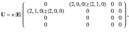${\bf U} = e \,\vert{\bf E}\vert \left( \begin{array}{cccc} 0&\lan... ...2,1,0\vert\,z\,\vert 2,0,0\rangle&0&0&0\\ 0&0&0&0\\ 0&0&0&0 \end{array}\right),$ \ref{665}

where the rows and columns correspond to the $ \vert 2,0,0\rangle$ , $ \vert 2,1,0\rangle$ , $ \vert 2,1,1\rangle$ , and $ \vert 2,1,-1\rangle$ states, respectively. Here, we have made use of the selection rules, which tell us that the matrix element of $ z$ between two hydrogen atom states is zero unless the states possess the same $ m$ quantum number, and $ l$ quantum numbers that differ by unity. It is easily demonstrated, from the exact forms of the $ 2s$ and $ 2p$ wavefunctions, that

$ \langle 2,0,0\vert\,z\,\vert 2,1,0\rangle = \langle 2,1,0\vert\,z\,\vert 2,0,0\rangle = 3\,a_0.$ \ref{666}

It can be seen, by inspection, that the eigenvalues of $ {\bf U}$ are $ \lambda_1= 3\,e\,a_0\,\vert{\bf E}\vert$ , $ \lambda_2 = - 3\,e\,a_0\,\vert{\bf E}\vert$ , $ \lambda_3=0$ , and $ \lambda_4 =0$ . The corresponding eigenvectors are

$ {\bf x}_1$ $ = \left( \begin{array}{c} 1/\sqrt{2} \\ 1/\sqrt{2} \\ 0 \\ 0 \end{array} \right),$ \ref{667} $ {\bf x}_2$ $ = \left( \begin{array}{c} 1/\sqrt{2} \\ - 1/\sqrt{2} \\ 0 \\ 0 \end{array} \right),$ \ref{668} $ {\bf x}_3$ $ = \left( \begin{array}{c} 0 \\ 0 \\ 1 \\ 0 \end{array} \right),$ \ref{669} $ {\bf x}_4$ $ = \left( \begin{array}{c} 0 \\ 0\\ 0 \\ 1\end{array} \right).$ \ref{670}

It follows from Section 7.5 that the simultaneous eigenstates of the unperturbed Hamiltonian and the perturbing Hamiltonian take the form

$ \vert 1\rangle$ $ = \frac{\vert 2,0,0\rangle + \vert 2,1,0\rangle}{\sqrt{2}},$ \ref{671} $ \vert 2\rangle$ $ = \frac{\vert 2,0,0\rangle - \vert 2,1,0\rangle}{\sqrt{2}},$ \ref{672} $ \vert 3\rangle$ $ = \vert 2,1,1\rangle,$ \ref{673} $ \vert 4\rangle$ $ = \vert 2,1,-1\rangle.$ \ref{674}

In the absence of an electric field, all of these states possess the same energy, $ E_{200}$ . The first-order energy-shifts induced by an electric field are given by

$ {\mit\Delta} E_1$ $ = +3\,e\,a_0\, \vert{\bf E}\vert,$ \ref{675} $ {\mit\Delta} E_2$ $ = -3\,e\,a_0 \,\vert{\bf E}\vert,$ \ref{676} $ {\mit\Delta} E_3$ $ = 0,$ \ref{677} $ {\mit\Delta} E_4$ $ = 0.$ \ref{678}

Thus, the energies of states 1 and 2 are shifted upwards and downwards, respectively, by an amount $ 3\,e\,a_0\, \vert{\bf E}\vert$ in the presence of an electric field. States 1 and 2 are orthogonal linear combinations of the original $ 2s$ and $ 2p(m=0)$ states. Note that the energy-shifts are linear in the electric field-strength, so this is a much larger effect that the quadratic effect described in Section 7.4. The energies of states 3 and 4 (which are equivalent to the original $ 2p(m=1)$ and $ 2p(m=-1)$ states, respectively) are not affected to first order. Of course, to second order the energies of these states are shifted by an amount that depends on the square of the electric field-strength.

Note that the linear Stark effect depends crucially on the degeneracy of the $ 2s$ and $ 2p$ states. This degeneracy is a special property of a pure Coulomb potential, and, therefore, only applies to a hydrogen atom. Thus, alkali metal atoms do not exhibit the linear Stark effect.

Contributors

Richard Fitzpatrick (Professor of Physics, The University of Texas at Austin)

$ \newcommand {\ltapp} {\stackrel {_{\normalsize<}}{_{\normalsize \sim}}}$ $\newcommand {\gtapp} {\stackrel {_{\normalsize>}}{_{\normalsize \sim}}}$ $\newcommand {\btau}{\mbox{\boldmath$\tau$}}$ $\newcommand {\bmu}{\mbox{\boldmath$\mu$}}$ $\newcommand {\bsigma}{\mbox{\boldmath$\sigma$}}$ $\newcommand {\bOmega}{\mbox{\boldmath$\Omega$}}$ $\newcommand {\bomega}{\mbox{\boldmath$\omega$}}$ $\newcommand {\bepsilon}{\mbox{\boldmath$\epsilon$}}$